
4 Statistical Evaluation of Difference
Chris Bailey, PhD, CSCS, RSCC
Generating and testing a hypothesis is a big part of the scientific process discussed in Chapter 1. The scientific process (often referred to as the scientific method) requires the development of a research based scientific guess, which is better known as a hypothesis. A hypothesis is a statement of an assumed relationship between variables or lack thereof. From there, we can create an experiment that will evaluate this hypothesis. Most of our experiments are actually set up to disprove a hypothesis. The experiment must have an inferential statistical test to evaluate that hypothesis. Then we compare the results of the experiment to the research hypothesis. If it disagrees, then the hypothesis was wrong. If it agrees, we do not immediately jump to the conclusion that the hypothesis was correct. We must repeat the experiment several times in different environments before jumping to that conclusion.
In order to test a hypothesis, it must actually be testable. This is often done with statistical tests comparing one condition to another condition (or conditions) that has been altered in some way that is consistent with the hypothesis. If there is a difference between the two conditions, the hypothesis may have been supported. This chapter will discuss many of these statistical tests.
Chapter Learning Objectives
- Learn about hypothesis generation and differentiate between types of hypotheses
- Understand statistical significance and probability
- Learn, implement, and interpret various types of statistical tests of difference
- Understand how sample size impacts statistical significance results
Hypothesis Generation and Different Types
When speaking of hypotheses, we have 2 main forms. The null hypothesis, or H0, is a statement that there is no relationship between 2 or more variables. Here it is important to remember that the term relationship acts like a continuum. So, it could mean that the variables are similar or different. So, a null hypothesis would be saying that there is no similarity or no difference between the variables in question (depending on the type of test run). The alternative hypothesis is the opposite. It states that there is some relationship (again a similarity or a difference) between the variables in question. The alternative hypothesis is generally notated by H with a subscript of 1, but can be H and any number if we have more than one hypothesis.
It is important to remember that our hypotheses must be testable or what may also be called falsifiable. This is actually why we use null hypotheses. Our hypotheses must be capable of being falsified by experimentation and/or observations. This notion was first described by Karl Popper early in the 20th century[1]. Consider an example where a physical therapist (PT) wants to evaluate a new form of ultrasound treatment and recovery times in clients compared to other forms of physical therapy all of which are recovering from ACL reconstruction using a similar patellar tendon graft technique. This hypothesis can be tested by randomizing placing all post-operative ACL patients into the new treatment group or another group and then comparing their length of recovery. How would the PT in our example set up a hypothesis that is falsifiable? Using the null hypothesis they might say that there will be no statistical difference in recovery times based on the modalities used. Is this falsifiable? Yes, because there might actually be a difference. What if the PT instead had the hypothesis that the new ultrasound treatment was the main reason why their clients are getting better compared to other PTs who don't use this modality? Is that falsifiable? No, because there are too many other variables that need to be accounted for (different PTs with different training and experience, different standards of care, other treatments used in conjunction with this treatment, etc.).
Popper went on to describe work that uses non-falsifiable hypotheses as pseudoscience and those that are falsifiable as science. Pseudoscience often seeks to confirm ones beliefs, whereas science seeks to disconfim first. Pseudoscientific claims struggle to hold their ground when held to the standard of scientific scrutiny.[2]
Statistical Significance
Whenever we complete statistical analyses, we should be looking for a measure of significance. There are two main ways to report and interpret significance. One of those, statistical significance, will be discussed here. The other, practical significance or meaningfulness, will be discussed later in the chapter on effect sizes.
Statistical significance is a measure of the reliability of our finding. It helps to the answer the following question of how probable was it that we found what we found? Or, if we ran the test again at a similar time with a similar sample, should we expect to find the same result? Alpha values will be used to help answer these questions. Alpha values or p values should be used to help us interpret our results. They represent the chance that we will commit a type 1 error where we reject the null hypothesis when we shouldn’t have. As a reminder, the null hypothesis states that there is not difference or no relationship depending on the type of test run. So, we would be committing a type 1 error if the null is rejected and state that there was a difference between the groups tested when there wasn’t. The p value indicates our probability of committing this error. It is widely accepted that a p value needs to be ≤ 0.05 to be statistically significant. So if a p value of 0.05 was found, we can statistically say that the average person in a given population (that the sample was taken from) will perform in this manner and there is less than a 5% chance that we are making an incorrect decision in rejecting the null hypothesis. If the p value was 0.25, that chance of error increases to 25%. Multiplying the p value by 100 will give the probability as a percentage that rejecting the null is the incorrect decision. Fortunately for us, we do not have to compute these values by hand. Most statistical software will compute this for us fairly quickly.
Alpha values are strongly influenced by sample size. With a large sample we might find that there is a statistically significant difference between 2 groups even if that difference is actually very small from a practical perspective. If we had a small sample, the difference would need to be quite a bit larger to achieve statistical significance. This idea will be expanded upon towards the end of this chapter. Knowing this information, some researchers might find a p value that is slightly higher than their chosen cutoff for statistical significance and seek to improve it by adding a few more subjects to the sample increasing its size. Assuming the same effect size, this would improve their chances of achieving statistical significance, but this is considered a violation of research ethics. You should have your methods planned out ahead of time and adding a few more subjects to your study after the fact is not acceptable. This practice is often called “p hacking” and there is evidence that it is quite common. For example, in the study by Head and colleagues, fields of science such as biology and psychology publish far more studies reporting p values less than 0.05 than they do above it, which is statistically improbable.[3]
Statistical Significance and Error Types
Type I and type II errors both occur when we make an incorrect decision about the results. A common way to describe this comes from an older comic that shows a physician giving his male patient the news that he is pregnant. This is obviously incorrect as males cannot carry children and this would be a type 1 error, since it concludes something is there when it isn’t. A type II error is the opposite. The same comic depicted this by showing an obviously pregnant female that is in labor receiving the news that she is not pregnant. This is a type II error because it concludes that something isn't there when it actually is.
A more realistic example for kinesiology would be that we incorrectly conclude that there is difference between the activity levels of seniors and middle-aged adults (age 40-65), measured by a smart watch from 9:00 am to 5:00 pm. There are many factors that could mislead us here, but one big one is that it only collects data in a specific time range and people that are active before or after those times will not be measured. We could be comparing active retired seniors to corporate office employees. If the middle-aged adults are more active before or after the traditional workday hours, this won’t be measured. This could lead to us thinking a statistical difference exists, but it doesn’t which would be a type I error.
Difference Tests
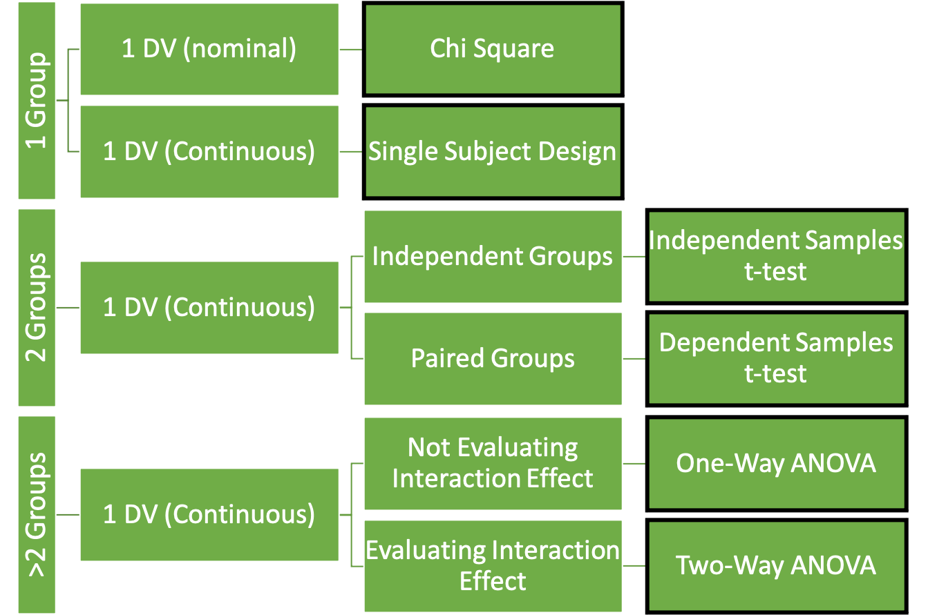
They type of variables used (along with the question we are trying to answer) will point us in the direction of which statistical test to use. Inspired by Vincent and Weir's decision tree style presentation of statistical test selection,[4] Figure 4.1 was created as a "cheat-sheet" for selecting an the appropriate statistical test when evaluating for difference. In the first column of the figure, we see group numbers and the test that should be run associated with each. So the first criteria that needs to be determined when selecting a test is the number of groups that are included in the sample. Next is the type of data that the dependent variable includes. While it is possible to have more than one dependent variable in a means comparison design, most will just run the same test multiple times on the different variables. As a result, Figure 4.1 only includes test that evaluate one dependent variable at a time.
Tests for only 1 group
Chi Square
If the dependent variable is nominal and only one group is included, the chi square test should be used. The chi square test can be used when only one group is being considered and dependent variable are nominal. For example, the COVID-19 pandemic forced nearly all college courses to transition to an online delivery form. Many students preferred this, but many also did not. Of course, those who feel strongly one way or the other are the ones that are most likely to speak up and they may not be the best representation of what students desire going forward. This could be tested by offering the same course in the traditional in-person and online formats during the same semester and then completing a chi square analysis on the resulting enrollment counts for each course.
The chi square is a test that evaluates the observed and expected frequencies of a given event. Using the equation below, we can see how to compute a single chi squared (X2) statistic.
[asciimath]X^2 = ("Observed Frequency" - "Expected Frequency")^2/"Expected Frequency"[/asciimath]
It is pretty simple, you subtract the expected value from the observed value, square it, and then divide that by the expected value. This can easily be done by hand. Where it could get complicated is when we have multiple instances to add. Our example is pretty easy, so it can be shown both ways.
| Class_type | students_enrolled | students expected | X2 |
|---|---|---|---|
| in_person | 107 | 124 | 2.33 |
| online | 141 | 124 | 2.33 |
| Total | 248 | 248 | 4.66 |
You can see the results in Table 4.1 above. A total of 248 students signed up for the course with 107 in the traditional course offering and 141 in the online offering. Assuming that each student could pick whichever format they want and there was not bias, we should expect that half of them (124) would select each format. This data will help us calculate the individual chi square statistics for each format. In order to do that we can plug our values into the equation shown earlier.
[asciimath]X_"in person"^2= (107-124)^2/124=2.33[/asciimath]
[asciimath]X_"online"^2 = (141 - 124)^2/124 = 2.33[/asciimath]
Interestingly, our two formats have the same X2 value because their differences between observed and expected are both 17 (X2in_person is actually -17, but that won't matter when it is squared). But our question was is there some form of bias overall based on formats offered. To determine that, we would add all of our X2 values together to create a combined chi squared statistic. We could then consult a chi squared distribution table to determine the value required to be statistically significant at the 0.05 alpha level.
[asciimath]X_"combined"^2 = 2.33 + 2.33 = 4.66[/asciimath]
Fortunately, we can accomplish all of these steps with the help of statistical software. Please download the dataset used in the tutorials below if you'd like to follow along.
Chi Square Analysis in MS EXCEL
In order to complete this in MS Excel, the data need to arranged similarly to Table 4.1 above. Excel has a built in function called CHISQ.TEST that will perform the chi square analysis and return a p value. If the p value is less than 0.05, then we would say that there is a statistical difference based on what was observed and what was expected.
=CHISQ.TEST(Actual_range,Expected_range)
If you are following along with the provided dataset, this will actually be =CHISQ.TEST(B2:B3,C2:C3). Recall that you do not have to type this in. You can use Excel's insert function button instead. This results in a p value of 0.031. This is less than 0.05, so we can say that teams playing in the initial season of a new stadium do perform differently than would be expected. Excel has a function to calculate the X2 statistic also.
=CHISQ.INV.RT(probability,deg_freedom)
In this function, the probability is the p value that was just found. The deg_freedom is the degrees of freedom, which is the number of categories minus 1. There are 2 categories in our example, so the deg_freedom = 1). This leaves us with a X2 statistic of 4.661, nearly identical to what was calculated by hand above.
Chi Square Analysis in JASP
| χ² | df | p | |||||
|---|---|---|---|---|---|---|---|
| Multinomial | 4.661 | 1 | 0.031 | ||||
Single-Subject Designs (SSD)
There are many single-subject designs can also be complete with only one group, the only caveat is that the group is made up of one individual (hence the name). Kinugasa, Cerin, and Hooper (2004) did an excellent job of explaining many of the available options here.[6] Bill Sands has also completed a significant amount of work in this area.[7] This textbook is largely focused on group designs, so these will not be discussed here, but those who are interested are encouraged to investigate further. These methods are especially important for those who wish to pursue careers in sport science.
Tests for 2 groups
Independent Samples t-test
Consider an example where you are working as an analyst in the front office of an NFL team. You want to determine if the style off offensive play has changed in the past decade compared to the previous one. Specifically, you want to look at the quarterback yards per game because you think it has increased. Again, you can have a null or an alternative hypothesis.
Here you can take a look at the data for the past 2 decades which includes the mean passing yards per game by year by NFL quarterbacks. With a t-test, 2 groups can be compared to evaluate whether there is a statistical difference between the 2001-2010 and 2011-2020 season data. An independent samples t-test will be needed to evaluate this, meaning that the groups are independent of one another. If it was the exact same quarterbacks in each decade, we would use a dependent samples t-test. Since none of the 32 teams would have had exact same QB for 20 years, this should be ran this as an independent samples t-test. Do you think there is a difference? Let’s take a look from a statistical perspective.
Independent Samples t test in MS Excel
The T.TEST function in Excel will be used to help answer this question. It takes 4 arguments. The first 2 are the data from the 2 groups being compared. The 3rd argument is the number of tails to be expected. If it was only expected that the values would change in 1 direction, a one-tailed test could be used. Since that is pretty rare in our research, a two-tailed test will generally be the best choice. The choice can be entered as either 1 or 2, indicating the number of directions the data might vary. The 4th argument is the type of t-test to be run. A value of 1 indicates that it is a dependent or "paired" samples test. This is not what we want here as the groups are not made up of the same members in each decade. A value of 2 should be used when an independent samples t-test should be run and we are assuming each group has equal variance. A value of 3 is entered when an independent samples t-test should be run and we are not assuming each group has equal variance. Tests of variance equality will be discussed more later on, so equal variance will be assumed here (2).
=T.TEST(array1, array2,tails,type)
=T.TEST(B2:B11,B12:B21,2,2)
As you can see from the data and from the arguments in the function above, B2:B11 represents the first array and the QB data from 2011-2020. QB data from 2001-2010 is in the second array (B12:B21). If these were set up as separate columns, the array information would need to be altered so that it selects the correct cell range. The result should read something like 4.71613E-08. Recall that we've seen values like this before and that this is a very small number. We can change the value to a number format at alter the number of digits shown to 3 to reveal a p value of less than 0.000. This shows that there is a statistical difference between the 2 decades in terms of passing yards per game and indicates that current teams are relying more heavily on the passing game than they did previously. But how big is this difference in practical terms? That will be discussed in the next chapter.
Independent Samples t test in JASP
In order to complete this analysis in JASP, a grouping variable will need to be created. This can be done manually by opening the .csv file and adding a variable called group with years 2001-2010 labeled as "older" adn 2011-2020 labeled as "newer." Alternatively, this column can also be computed in JASP. Simply click the + icon to create a new variable and give it a name. Then click on the hand pointer icon to use JASP's drag and drop method. In order to do this we will create a logical expression, which will result in computing variable values as either "True" or "False." Drag the Year variable into the formula builder. Now select the ≥ symbol and type 2011. Your formula should read as "Year ≥ 2011." Click compute and the data should be populated. Seasons between 2011 and 2020 should have a "True" label and earlier seasons should have a "False" label.
Now that we have a grouping variable, click on T-tests and select the Classical Independent Samples T-Test option. Move the Y/G variable into the variables box[8] and the group variable (or whatever variable name you created) into the grouping Variable box. The results should now be populated and should look like Table 4.3 below. By adding Descriptives options into the results we can see that the more recent decade produces higher values of Y/G than the previous decade. Along with the p value being below 0.05, this shows that there is a statistical difference between the 2 decades in terms of passing yards per game and indicates that current teams are relying more heavily on the passing game than they did previously. But how big is this difference in practical terms? That will be discussed in the next chapter.
| t | df | p | |||||
|---|---|---|---|---|---|---|---|
| Y/G | -8.959 | 18 | < .001</td> | ||||
| Note. Student's t-test. | |||||||
Dependent Sample t-test (paired)
What if you wanted to test the same group at 2 different time points? Or if you wanted to test the same subjects on 2 different devices to compare the devices? In that case, we would use a paired or dependent samples t-test. It is the same group, but it counts as 2 since they are tested twice.
Let’s stick with our NFL example, but we will now look at QB development in terms of passing yards per game. If we are looking at development, we need to track the same QBs over time. So we have a sample of QBs that played prior to 2010 and after. We can again test this with a t-test, but it will now need to be a paired t-test since the same members are in each group. Let’s take a look at our data.
Here is the example data for the same group tested twice. Unlike the previous data, we are now using theoretical data to make sure we had enough data points. Now you can see an alternative way to structure your data from what we used previously. Here each group is set up as its own column. Many prefer this method, but again it is up to you.
Dependent Samples t test in MS Excel
The process for completing a paired samples t test in Excel is almost identical to the independent example above. But now the final argument will need to have a value of 1 instead of 2 to tell Excel that the data are paired.
=T.TEST(B2:B11,C2:C11,2,1)
Take note that the dataset structure has now changed, so array 2 now appears next to array one in column C. Also note that the final argument has been changed to 1. Recall that you are not expected to remember all of the arguments. Click the function/formula builder icon and Excel will walk you through it.
The resulting value should be a p value of 0.024 again indicating that there is a statistical difference between the 2 groups.
Dependent Samples t test in JASP
The data set format for a paired samples test in JASP is different than what we have used before. Now each group should be set up as its own column. This has already been done for you in the attached dataset. In order to run a dependent samples t test in JASP, simply click on T-Tests and select the Paired Samples T-Test Classical option. Now move the two variables over into the variable pairs box ("Pre 2010" and "Post 2010"). The results should look similar to Table 4.4 and 4.5 below. Select Descriptives again and we can see that there is a statistical difference between the pre 2010 data and the post 2010 data, with the post 2010 data being higher (p = 0.024).
| Measure 1 | Measure 2 | t | df | p | |||||||
|---|---|---|---|---|---|---|---|---|---|---|---|
| Pre 2010 | - | Post 2010 | -2.717 | 9 | 0.024 | ||||||
| Note. Student's t-test. | |||||||||||
| N | Mean | SD | SE | ||||||
|---|---|---|---|---|---|---|---|---|---|
| Pre 2010 | 10 | 224.600 | 20.184 | 6.383 | |||||
| Post 2010 | 10 | 251.100 | 25.370 | 8.023 | |||||
Tests for more than 2 groups
Whenever there are more than 2 groups, some form of an ANOVA will need to be used to. ANOVA stands for analysis of variance. There are 2 common types, we will run the first when we have 1 nominal variable but has more than 2 groups. It is called a one-way ANOVA. The second type is called a two-way ANOVA and it is used when have more than one nominal IV and we expect an interaction effect between them.
As an example, imagine that you need to determine the most effective method of increasing strength as measured by the bench press using a 1 repetition max test. You have 3 groups, and each will only perform exercises that match their training method of either free weights, machines, or bodyweight exercises. You cannot run a t-test if you have more than 2 groups. Here you mustl run a one-way ANOVA to determine if there is a statistical difference between the groups. Keep in mind that this will tell you if there is a difference between the groups but won’t tell you which of the groups differ with which. You will have to run a post-hoc test to determine that.
Here is the data for this example. Notice that we are again including a column for the training method, or group. The other column includes the 1RM bench press values in kilograms. If your data are set up as a column for each group, instead of having a grouping column like you see here, most statistical programs will not be able to run it. So, you should always set up your data in this nice and tidy format. Each row is a single observation, and every column is a variable. Unfortunately, one program that cannot run and ANOVA this way is MS Excel. MS Excel requires each group to have data separated into columns similar to what can be observed in Table 4.6 below.
| Group_1 | Group_2 | Group_3 |
|---|---|---|
| value | value | value |
| value | value | value |
| value | value | value |
| value | value | value |
One-way ANOVA in MS Excel
The first step in completing a one-way ANOVA in Excel is to rearrange the data into the format described above in Table 4.6. This can be completed by copying and pasting fairly easily. Using the Data Analysis Toolpak, select Anova: Single Factor. For the input range, you will need to include all of the data and the variable headings from the first row. Make sure to check that labels are in the first row. By default, 0.05 will be used for the alpha value. Similar to the regressions completed earlier, you will need to select where the result are to be displayed. After clicking OK, the results should look similar to those of Table 4.7 and 4.8 below (some rounding was applied before inserting here).
| SUMMARY | ||||
|---|---|---|---|---|
| Groups | Count | Sum | Average | Variance |
| free_weights | 10 | 1316 | 131.6 | 375.6 |
| machines | 10 | 1131 | 113.1 | 332.1 |
| bodyweight | 10 | 839 | 83.9 | 223.2 |
| ANOVA | ||||||
|---|---|---|---|---|---|---|
| Source of Variation | SS | df | MS | F | P-value | F crit |
| Between Groups | 11567.2667 | 2 | 5783.633 | 18.639 | 0.000 | 3.354 |
| Within Groups | 8378.2 | 27 | 310.304 |
Table 4.7 shows the summary descriptive statistics and we can see from that that each group had 10 members and free weights had the highest average 1RM value. Table 4.8 displays the ANOVA results. The p value is less than 0.05, so there is a statistical difference between at least 2 of the groups. The f statistic and the f critical value are both used to determine statistical significance. The f crit value shows that an f statistic of 3.354 is required to be statistically significant at the alpha value selected (p = 0.05).
Unfortunately, the ANOVA does not inform us of which groups are different from which. In order to determine that, a post-hot test must be performed. Excel does not have a function to do this along with the ANOVA, so these must be completed in a separate step. There are many post-hoc test options with other statistical software, but those would have to be caluclated by hand in MS Excel. Instead, most will now run independent samples t test between each group to see where the statistical difference lies. See below for more information on this step and why it is necessary.
One-way ANOVA in JASP
After opening the data in JASP and verifying that the data types are correct, click the ANOVA drop-down menu and select the classical form of the ANOVA. Now move the 1RM_Bench variable into the dependent variable box (note that this variable may have been renamed in JASP to start with a "V" because variables are not allowed to begin with a number). Now move the grouping variable Training_Method into the fixed factors box.
| Cases | Sum of Squares | df | Mean Square | F | p | ||||||
|---|---|---|---|---|---|---|---|---|---|---|---|
| Training_Method | 11567.267 | 2 | 5783.633 | 18.639 | < .001</td> | ||||||
| Residuals | 8378.200 | 27 | 310.304 | ||||||||
| Note. Type III Sum of Squares | |||||||||||
Table 4.9 shows that there is a statistical difference with a p value of less than 0.01 based on the training method used. But it does not show which groups are different from which. In order to determine that, a post-hot test must be performed. Fortunately, this is just another button click away in JASP. Scroll down to the Post-Hoc Tests menu and click to expand it. Now move the grouping variable (Training_Method) over and make sure that the Tukey correction is selected. The Tukey HSD or honestly significant difference is they type of post-hoc test that will be used. There are other options that may be used in different situations. The results should now be displayed. You may also wish to see a plot of the results and this can be added by changing the selections in the descriptives plots menu.
|
Post Hoc Comparisons - Training_Method |
|||||||||||
|---|---|---|---|---|---|---|---|---|---|---|---|
| Mean Difference | SE | t | p tukey | ||||||||
| bodyweight | free_weights | -47.700 | 7.878 | -6.055 | < .001</td> | ||||||
| machines | -29.200 | 7.878 | -3.707 | 0.003 | |||||||
| free_weights | machines | 18.500 | 7.878 | 2.348 | 0.066 | ||||||
| Note. P-value adjusted for comparing a family of 3 | |||||||||||
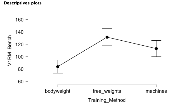
Table 4.10 displays the between group comparisons and their associated p values. When bodyweight is compared to free weights, a p value of less than 0.001 is found, so these groups are statistically different. The same is true when comparing bodyweight to machines (p = 0.003). Free weights were not statistically different from machines, but it was close (p = 0.066). This demonstrates that bodyweight training should not be the training method used when seeking to increase 1RM bench press when other options like free weights and machines are available. It may also indicate that free weights are the best option, but they were not statistically different from machines in this sample.
Post-Hoc (after the fact) Tests
Hopefully you are now thinking if we have to run a post-hoc test, which could be t-test afterward, why not run it from the beginning and not waste our time with the ANOVA. That is a great question. The reason we must run the ANOVA first is that it protects us from making a type I error. The more tests or comparisons we run, the more likely we are to find something by random chance. If we thought we found a difference when when it was actually just a random chance occurrence, we would be making a type I error.
Explained another way – Imagine I offer you a way to earn some extra credit in your college course. For this example, I have a 2 feet by 5 feet table, a hammer, and a blindfold. I will offer you 1 whole percentage point. In order to receive this point, you must place your phone on the table and I get to swing the hammer at the table while blindfolded. I won’t know where you placed the phone on the the table since I’m blindfolded, so this would be random chance if I happen to hit it.
Would you do it for one percentage point? If the average phone is 2.5 inches wide by 6 inches tall, there is only a 1 and 96 chance that I will hit your phone (~1%). Those are pretty good odds in your favor. What if I swing and miss and I now offer you another percentage point if

I can swing again and you can move your phone to a new location on the table. I assume you may be worried that I might be learning where you phone is not located after each swing. The odds are still the same, 1/96. Would you let me do it? How many swings would you let me take if you kept getting a full percentage point?
Your answer would probably depend on your current grade, but you would probably let me take a handful of swings. If we ignore the fact that your grade could reach a point where it meets your needs, why would you stop me from swinging. Even though the odds of each individual swing are low, 1 in 96, they increase with each swing. In fact, after swing 48, I would become more likely to hit your phone than not. As you can see, the more chances you offer the more likely I will hit something by random chance. The same is true with statistical comparisons. The more we run, the more likely we are to randomly find something. This is why running the ANOVA first is beneficial. It limits the number of comparisons run. If we do not find statistical difference in the ANOVA, we do not need to run any more comparisons, which would be less than running a bunch of individual comparison tests.
More than 2 groups and 2 independent variables
Our last form of means comparison is likely our the complicated one, but it’s not that bad. It is essentially the same as the one-way ANOVA, only we have another independent variable that might interact with the other independent variable. In the previous example, we looked at training methods and strength level. Do you think there might be other variables that impact strength? There definitely are. What about training background or training age? We’ll look at examining both of these with a two-way ANOVA example.
In this example we are testing the vertical jumping performance of undergraduate kinesiology students. Along with training method, we will also look at training age. Each student is classified as either (high ≥ 2 years of training) or low (< 2 years of training). They are also classified as either using resistance training with weightlifting movements or resistance training without weightlifting movements.[9] So, one of our groups will incorporate weightlifting movements or their derivatives (hang clean, jump shrug, etc.) Similar to all previous tests, either null or alternative hypotheses may be used, but we must have one for each nominal variable and for the combination. So, if we are using the null, our hypotheses would be the following:
- There is no difference between training age groups
- There is no difference between training methods
- There is no interaction effect of training age and training method
Here's the data if you'd like to follow along. Note that there are 3 columns in the data. First is the jump performance, measured as jump height (in m) for all subjects. Next, is the first nominal or grouping variable, training age. And finally, we see the training method used. There are 40 subjects in this dataset. The first 10 subjects are in the higher training age category and use weightlifting movements. The next 10 subjects are in the higher training age category, but do not use weightlifting movements. The 3rd set of 10 is in the lower training age but does utilize weightlifting movements in training. Finally, the last 10 is in the lower training age category and does not use weightlifting movements. Now that you better understand the data setup, let's take a look at the analysis.
Two-way ANOVA in MS Excel
Frustratingly, Excel requires yet another different format to perform a two-way ANOVA. Similar to the one-way ANOVA, one variable must be divided into 2 columns by one of the grouping variables. But a two-way ANOVA has 2 independent variables, so a 3rd column should be used to describe each observation by the new group. This manipulation has already been completed for you and you can download it here. Here is a sample of the format if you'd like to get some practice in altering the format. This format is somewhat of a combination of the two formats described.
| Independent Variable #2 | Independent Variable #1 Group 1 | Independent Variable #1 Group 2 |
|---|---|---|
| Group A | numerical value | numerical value |
| Group A | numerical value | numerical value |
| Group B | numerical value | numerical value |
| Group B | numerical value | numerical value |
The two-way ANOVA can be completed with the Data Analysis Toolpak and it is called "Anova: Two-Factor with Replication" in the options. Similar to the one-way ANOVA, you will need to select the entire range of the data including the variable headings. Interestingly, you do not need to let Excel know that variable headings are used this time. If you recall from the data set up, we have 40 subjects that are essentially divided into groups of 10. As a result, 10 must be entered into the Rows per sample box. This shows another issue with MS Excel in that the data need to be sorted so that each group or sub-sample must be arranged together. Excel will not be able to differentiate them by their grouping variable values like other programs can. Your data are already set up in this way. Next, select where the results should be placed and select OK.
The first 2 tables of the Excel output will be summary statistics for each group and variable. The last table output will be the two-way ANOVA results.
| ANOVA | |||||||
|---|---|---|---|---|---|---|---|
| Source of Variation | SS | df | MS | F | P-value | F crit | |
| Sample | 0.112 | 1 | 0.112 | 24.011 | 0.000 | 4.113 | |
| Columns | 0.161 | 1 | 0.161 | 34.468 | 0.000 | 4.113 | |
| Interaction | 0.038 | 1 | 0.038 | 8.215 | 0.007 | 4.113 | |
| Within | 0.168 | 36 | 0.005 | ||||
| Total | 0.481 | 39 |
The term Sample in Table 4.12 refers to the variable that appears in the first column of the selection. In our case, that was Training_Age. The term Columns refers to the subsequent columns WL and non_WL. Knowing that, we see that there is a statistical difference between groups based on Training_Age (Sample) with a p value of less than 0.000. We do not need to do a post-hoc test here because there are only 2 groups in this variable (High and Low), so we already know where the difference is. Similarly, there is a statistical difference between training methods (Columns) with a p value of less than 0.000. Finally, we see there is also a statistically significant interaction effect (p = 0.007) between both independent variables. A post-hoc test would be necessary here to determine where the differences lie. In MS Excel, that means runing several (7) more independent samples t tests.
This can be confusing for those that do not use this on a regular basis. Excel's lack of intuitiveness, inconsistent required formats, and odd variable naming make this a less than desirable solution for running a two-way ANOVA. This is often the point where many abandon MS Excel for other statistical software if they haven't already.
Two-way ANOVA in JASP
A two-way ANOVA in JASP is pretty simple to run and very similar to the one-way ANOVA, but the interpretation adds in another level. The only difference is that you will now move two grouping variables into the fixed factors box. This means that Jump_Height will be in the dependent variable box and both Training_Age and Training_Method will be in the fixed factors box.
|
ANOVA - Jump_Height |
|||||||||||
|---|---|---|---|---|---|---|---|---|---|---|---|
| Cases | Sum of Squares | df | Mean Square | F | p | ||||||
| Training_Age | 0.112 | 1 | 0.112 | 24.011 | < .001</td> | ||||||
| Training_Method | 0.161 | 1 | 0.161 | 34.468 | < .001</td> | ||||||
| Training_Age ✻ Training_Method | 0.038 | 1 | 0.038 | 8.215 | 0.007 | ||||||
| Residuals | 0.168 | 36 | 0.005 | ||||||||
| Note. Type III Sum of Squares | |||||||||||
Table 4.13 shows that there is a statistical difference between groups based on Training_Age with a p value of less than 0.001. We do not need to do a post-hoc test here because there are only 2 groups in this variable (High and Low), so that is where the difference is. Similarly, there is a statistical difference between training methods with a p value of less than 0.001. The 3rd row shows that there is also a statistically significant interaction effect (p = 0.007) between both independent variables (labeled as Training_Age * Training_Method). A post-hoc test is necessary here to determine where the differences lie. That can be done by expanding the Post Hoc Tests menu and moving Training_Age * Training_Method over. Make sure Tukey is selected again.
|
Post Hoc Comparisons - Training_Age ✻ Training_Method |
|||||||||||
|---|---|---|---|---|---|---|---|---|---|---|---|
| Mean Difference | SE | t | p tukey | ||||||||
| High, WL | Low, WL | 0.044 | 0.031 | 1.438 | 0.484 | ||||||
| High, non_WL | 0.065 | 0.031 | 2.125 | 0.165 | |||||||
| Low, non_WL | 0.233 | 0.031 | 7.616 | < .001</td> | |||||||
| Low, WL | High, non_WL | 0.021 | 0.031 | 0.686 | 0.902 | ||||||
| Low, non_WL | 0.189 | 0.031 | 6.178 | < .001</td> | |||||||
| High, non_WL | Low, non_WL | 0.168 | 0.031 | 5.492 | < .001</td> | ||||||
| Note. P-value adjusted for comparing a family of 4 | |||||||||||
Here we can see that there are statistical differences between the high training age group that uses weightlifting methods and the low training age group that does not use weightlifting methods (p < 0.001). We also see differences between the low training age group that uses weightlifting methods and the low training age group that does not use weightlifting methods (p < 0.001). Finally, we see a difference between the high training age group that does not use weightlifting methods and the low training age group that does not use weightlifting methods (p < 0.001).
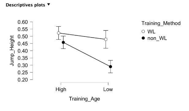
Again, plots can be added using the Descriptive Plots menu. Both independent variables can be added to the same plot with one going into the Horizontal Axis box and the other going into the Separate Lines box. This is demonstrated in Figure 4.4 below. When observing a descriptives plot such as this, an interaction effect can be spotted if the lines intersect or if they ever would intersect assuming the same slopes. Here we do see that as they likely would intersect if both lines were carried out further on the left side of the plot.
Sample size and Statistical Significance
Now that we have learned several different ways to make comparisons and seen how to get a p value for each, let’s revisit the topic of sample size. We learned earlier that sample size can influence our ability to achieve statistical significance. The larger the sample, the more likely we are to find a statistically significant finding. In order to further demonstrate this, please view one more file that includes 3 different datasets of jump heights that each have different sample sizes (10, 20, and 40). While the sample sizes differ, they are all normally distributed with the exact same mean and standard deviation. So, the actual magnitude of the difference between trials in each dataset will not change, only the sample size. Means comparison tests were run on each of the 3 datasets to show how p values will change when the sample size increases, even when the rest of the data stays the same. As you can see the p values get lower as the sample size increases.
This demonstrates an issue for small sample studies, but also shows another reason that we should not solely rely on p values. The ability to establish statistical significance is helpful to demonstrate the reliability of our findings, but the do not provide any information on the magnitude of difference (or relatedness) and they are heavily influenced by sample size. The next chapter on effect sizes will address part of this issue.
- Popper, K. 1932. The Two Fundamental Problems of the Theory of Knowledge. ↵
- Sagan, C. 1995. The Demon-Haunted World: Science as a Candle in the Dark. Random House, USA ↵
- Head et al., The Extent and Consequences of p-Hacking in Science, PLOS Biology, 2015 ↵
- Vincent, W., Weir, J. 2012. Statistics in Kinesiology. 4th ed. Human Kinetics, Champaign, IL. ↵
- If we had and alternative hypothesis where we expected another probability than 50% of the students to enroll in each format, you can alter those values by selecting the "Expected proportions" button under the Tests section. ↵
- Kinugasa T, Cerin E, Hooper S. Single-subject research designs and data analyses for assessing elite athletes' conditioning. Sports Med. 2004;34(15):1035-50. doi: 10.2165/00007256-200434150-00003. PMID: 15575794. ↵
- Sands, W. A., Kavanaugh, A. A., Murray, S. R., McNeal, J. R., & Jemni, M. (2017). Modern Techniques and Technologies Applied to Training and Performance Monitoring, International Journal of Sports Physiology and Performance, 12(s2), S2-63-S2-72. ↵
- Recall that one of the big benefits of using JASP is that you can run the same analysis on several variables at once. If we wanted to perform the same analysis on other variables besides Y/G, we could move those over now as well. ↵
- Side note: If you aren’t aware, weightlifting (spelled as one word) is the sport of weightlifting with the 2 lifts, snatch and clean and jerk. It is a very competitive sport internationally and we see it in the Summer Olympics. You may have incorrectly heard them called Olympic lifts or something similar because of this. This is incorrect because you don’t have to be in the Olympics to do these lifts. Imagine if we referred to swimming as Olympic Swimming. If weight lifting is spelled as 2 words, it is referring to the act of lifting weights, not the sport. ↵
Stemming from non-falsifiable claims and confirmation bias, it generally claims to be or portrays itself as scientific, but does not follow the scientific method.
When the null hypothesis is incorrectly rejected.
When we incorrectly accept the null hypothesis and state that there is no difference or potentially no relationship, when there actually is one.
outcome variable or the variable that the independent variable has some effect on
