
5 Practical Significance and Effect Sizes
Chris Bailey, PhD, CSCS, RSCC
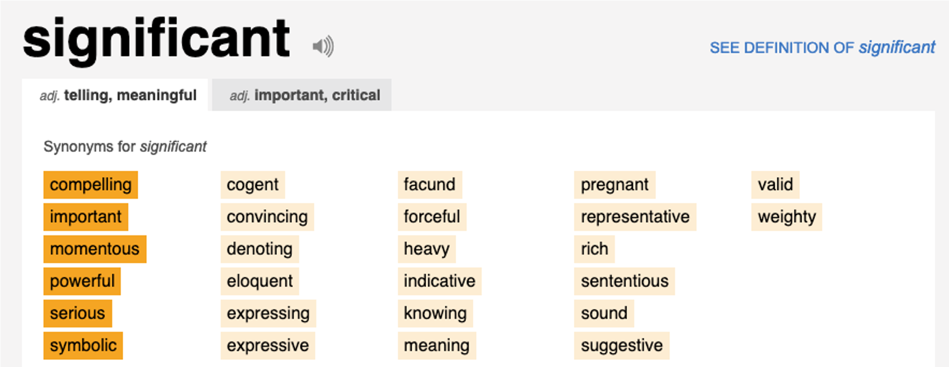
We have heard the phrase statistical significance used quite a bit already when we are discussing a statistical finding that has a p value of less than or equal to 0.05. Often in research and academic journal articles, the phrase statistical significance is shortened to just state that it was a "significant finding." This is problematic for many who don’t understand that the word significant in a statistical perspective may be different than the more straightforward and widely used definition for significance that most people use. For example, consider a study that demonstrates a statistically significant difference between weight loss outcomes in two groups. One that took a weight loss supplement and one that did not. This may be described as a ”significant” difference in outcomes between the groups because the p value was less than 0.05. Think about how the supplement company might use that for marketing purposes. They might say something like “lose significantly more weight with our product” or any of the other synonyms shown above that comes from thesaurus.com. But that isn’t exactly what statistical significance means. If we have a large enough sample, we can find a statistically significant difference even when that difference is a small one (demonstrated at the end of the last chapter). So, we should also be concerned with practical differences.
Another way to describe practical difference is meaningfulness. How meaningful is the statistical difference we found? This information is what is probably most important to the consumer or end user, but it might not be the easiest to spin for marketing. Whenever we perform statistical analyses, whether they are looking for similarity (i.e. correlation) or difference (i.e. t test or ANOVA), we should also include a measure of meaningfulness.
Meaningfulness can be quantified by effect size estimates. We will discuss two main types of effect sizes, one of which you are actually already familiar with.
Chapter Learning Objectives
-
Discuss meaningfulness as it applies to quantitative analysis
-
Learn how to quantify and interpret effect size estimates
Effect Sizes
Effect sizes, or more appropriately effect size estimates, help us statistically quantify practical significance. Effect sizes have also been described as a measure of "meaningfulness."[1] From a purely practical and applied perspective, the effect size should be the primary outcome of research inquiry.[2] No matter what we are measuring, we are likely most interested in the size of the difference or relatedness between variables. The reliability of our finding or how confident we are in the finding is important also, but it shouldn’t be the only product.
This has become such a problem in many fields of research that more than 800 researchers recently published a paper condemning the usage of p values since many rely too heavily on it and not enough on practical measures of significance that demonstrate realistic effects.[3] Completely abandoning measures of statistical significance like p values is probably a little too extreme, but their point is well taken. We should be publishing measures of both statistical and practical significance or meaningfulness.
So, let’s define effect size. An effect size is a measure that describes the magnitude or size of the difference or relatedness between the variables we are measuring. This means that it is describing the practical/meaningful significance. As we will see in this chapter, it really all boils down to how much the data overlaps between our groups or variables. If we are comparing groups for differences, we would likely not expect to see much overlap in the data. If we were evaluating our data for similarity or association, we are looking for more overlap.
Types of Effect Sizes
As mentioned above, effect sizes can be created for both relatedness and difference tests. This essentially means that there are 2 “families” of effect sizes; r for relatedness and d for difference. Conversions can also be completed between the two if it was necessary to make comparisons across different study types. That won't be demonstrated in this chapter, but a quick internet search for "r to d effect size conversion," or vice versa, will bring up several online calculators and formulas.
Cohen's d Effect Size Estimates
Looking on the difference side of effect sizes (ES), Cohen’s d effect size estimates are most commonly seen. They are named after Jacob Cohen. They can be quickly calculated when both means and the pooled standard deviation is known. The means can be from independent or paired groups. The pooled standard deviation is the standard deviation calculated from both groups as one.
[asciimath]"Cohen's d ES" = (M_1 - M_2)/"sd"_"pooled"[/asciimath]
[asciimath]M = mean, sd = "standard deviation"[/asciimath]
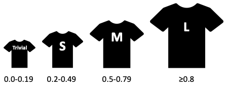
With this data, we simply subtract one mean from the other and divide by the pooled standard deviation. If the value is negative, that simply means that the second mean or the one that was subtracted from the other was larger than the original mean. This is dependent on how the dataset was ordered or how they were called into the formula. So, the direction doesn’t really matter here since the magnitude is the largest concern. For this reason, the negative sign is usually not included. Effect size estimates can be interpreted with the scale provided. Anything less than 0.2 is considered a trivial difference, 0.2 to 0.49 is a small difference, 0.5 to 0.79 is a medium difference, and anything ≥ 0.8 is a large difference.
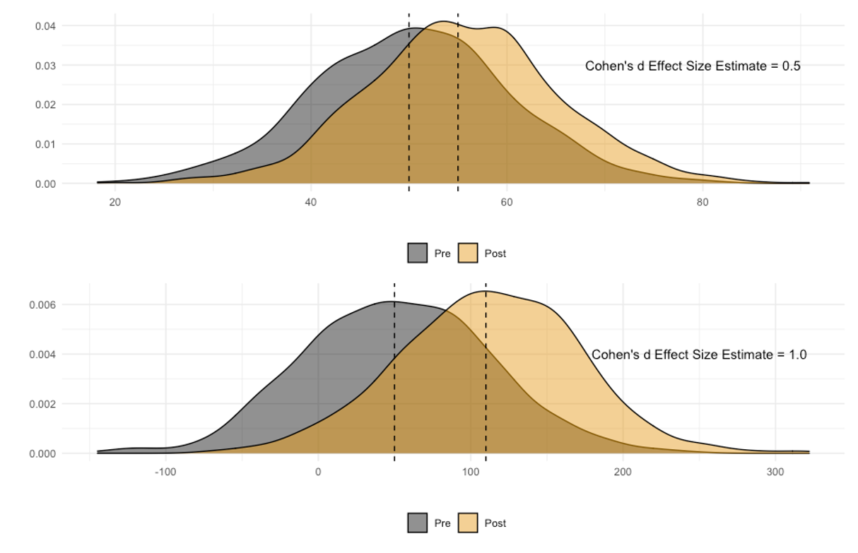
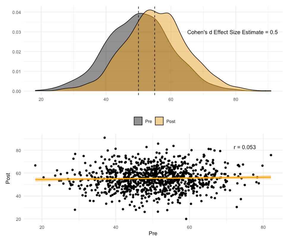
As mentioned previously, effect sizes really all boil down to the amount of overlap in the data. Figure 5.3 demonstrates this with 2 examples. The first one (on top) is a comparison of 2 groups. One distribution has a mean of 50, the other has a mean of 55, and the pooled standard deviation is 10. Solving for the Cohen’s d effect size, we find that there is a medium difference between these 2 groups with a value of 0.5 (d=(55-50)/10). The second example has a distribution with a mean of 50, a distribution with a mean of 110, and a pooled standard deviation of 60. Here we find a large difference with a Cohen’s d effect size of 1.0 (d=(110-50)/60).
Take a look at the amount of overlap between the distributions in each example. Can you see why the Cohen’s d effect size estimate is larger in the 2nd example? It has a lot less overlap between the distributions. What if the data distributions were completely separate with no amount of overlap? What would happen to the effect size then? It would increase quite a bit. What if nearly 100% of the data were overlapping? The effect size would shrink quite a bit and likely be trivial. This is of course if we are still using Cohen’s d as our measure of effect size, since it is looking for difference. But what if we wanted to look for similarity?
r Effect Size Estimates
When looking for similarity, the PPM r value should be used as an effect size. The fact that r is an effect size is a good thing, since we already know how to quantify it and use it from Chapter 3. Recall that r values can range from -1 to 0 to +1 and we have already seen how to interpret them in Chapter 3.
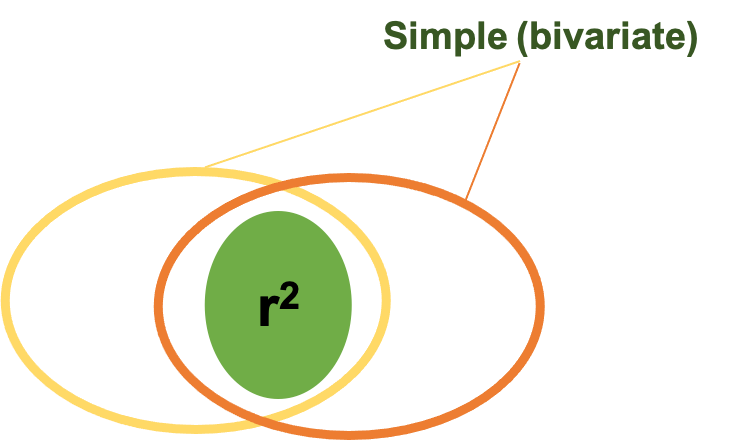
When interpreting effect sizes for relationships or associations, we are still concerned with the amount of overlap in the data, and we’ve seen this before in Figure 3.12 (now 5.4 in this chapter). When utilizing a bivariate correlation or simple linear regression with only 2 variables (which are represented by the ovals above), we are mostly concerned with the area where they have shared variance. That is represented as the area of overlap in this figure. Remember the coefficient of determination r2 helps us explain the amount of shared variance. Please review Table 3.4 (reproduced below) and go back to Chapter 3 if you need a refresher.
| r value | interpretation | r2 | % of variation |
|---|---|---|---|
| 0.0-0.09 | Trivial | 0.00-0.0081 | 0-0.81% |
| 0.1-0.29 | Small | 0.01-0.0841 | 1-8.41% |
| 0.3-0.49 | Moderate | 0.09-0.2401 | 9-24.01% |
| 0.5-0.69 | Large | 0.25-0.4761 | 25-47.61% |
| 0.7-0.89 | Very Large | 0.49-0.7921 | 49-79.21% |
| 0.9-0.99 | Nearly Perfect | 0.81-0.9801 | 81-98.01% |
| 1 | Perfect | 1 | 100% |
Going back to our previous example with Cohen's d in Figure 5.3, we see the first example that produced a Cohen’s d effect size estimate of 0.5 which is interpreted as a medium amount of difference between the variables. You might be thinking that you still see quite a bit of overlap in the data distributions. If there is a medium amount of difference between the variables, how much similarity is there? Intuitively, you might think that there is a medium amount of similarity, but that is incorrect as you can see in the scatterplot prodcued below the distributions (in Figure 5.5 below). In fact, it has a PPM r value of 0.053 which is considered a trivial amount of similarity. This demonstrates that difference and similarity are not necessarily on the same continuum. Just because there isn’t a large difference between two variables, they aren’t necessarily related.
This also demonstrates why we use specific data visualization techniques with each statistical test. Whenever you are testing for difference, you should likely use a box and whisker plot, density plot, or distribution plot. Whenever you are testing for similarity, you should use a scatterplot. If the wrong plot is used, you may confuse or mislead your audience.
Calculating Effect Sizes
Fortunately, our r values are already effect size measurements, so we don’t need to do anything else to them. However, whenever testing for difference, we still need to calculate Cohen’s d effect size estimates. These can be produced relatively easy in most statistical programs. Some are as simple as checking a box, but others may require the formula be typed in. As always, you can download the dataset if you would like to follow along with the tutorials below. This dataset includes performance data from jump testing, 30 yard sprints, and 1RM bench press. The sample was grouped based on bench press strength with those above 200 lbs in the "stronger" group and those below in the "weaker" group. This puts 10 into each group. An independent samples t test on the 30 yd sprint time variable produces a p value of 0.018, so we know there is a statistical difference between the 2 stronger and weaker groups. Calculating a Cohen's d effect size will help understand how meaningful this difference is.
Calculating Cohen's d in MS Excel
Unfortunately, there is no built-in function in Excel or option in the Data Analysis Toolpak for Cohen's d. So it must be calculated. If we go back to the equation (d=(M1-M2)/sdpooled), we know that we first need to calculate the means for each group and then the pooled standard deviation. MS Excel does have functions for those, so you can run each of those individually, or if you are looking for an added challenge, you can calculate them inside of the Cohen's d equation. Either way, make sure you use parentheses so that your order of operations does not alter your answer.
The mean of the weaker group should be 4.15 s and the mean of the stronger group should be 3.86 s. So we know that the stronger group also seems to be faster. The pooled standard deviation should be something close to 0.2837252 (using the =STDEV.S function). Remember do not round prior to calculating the final answer. This may alter your result. Instead of typing these values in, you should click each cell where the value is calculated. For example, my mean for the weaker group was calculated in F4, the mean for the stronger group was calculated in F5, and the pooled standard deviation in F6. So my formula was:
=(F4-F5)/F6
and this produced a Cohen's d effect size of 1.02 (rounded). If you wanted to do all the calculations in one cell the formula should read:
=(AVERAGE(E2:E11)-AVERAGE(E12:E21))/STDEV.S(E2:E21)
Either way should work, but there is more opportunity for error when combining multiple steps, so only attempt that if you are comfortable.
Calculating Cohen's d in JASP
A Cohen's d effect size (or several other types of effect size) can be added to any means comparison test by checking a box to do so. For t tests, this can be found under "Additional Statistics." After checking the Effect Size box, Cohen's d is already selected by default. Once checked, it appears in the tabular results output.
|
Independent Samples T-Test |
|||||||||
|---|---|---|---|---|---|---|---|---|---|
| t | df | p | Cohen's d | ||||||
| V30yd | -2.612 | 18 | 0.018 | -1.168 | |||||
| Note. Student's t-test. | |||||||||
If you also followed along with the solution in MS Excel, you may notice that the value is different. First, it's negative. This is because JASP used the stronger group as M1 instead of the weaker group as was done above. This simply means the sign is flipped and it can be dropped. The other difference between these values comes from how the pooled standard deviation was calculated. In Excel, it was a true pooled standard deviation since all the values were highlighted in the formula. Another way to calculate the sdpooled is by using an estimate equation where the square of each group's sd is added together, divided by 2, and then the square root of that value represents the sdpooled. This is how JASP calculates the sdpooled. This estimation is helpful for calculating a sdpooled when you don't have access to raw data, but do have access to group summary statistics as is often the case when reading a published article.
sdpooled = √((sd12 +sd22)/2)
Calculation of a Cohen's d for an ANOVA in JASP, is completed in the post-hoc stage. Again, the Effect Size box must be checked and it will be added to the post-hoc results output.
Other Types of Effect Sizes
There are quite a few other forms of effect sizes that can be used and should be with specific scenarios. Cohen's d and the PPM r value are the most common and they are the most widely understood, so it is easy to see why many prefer them. No matter what effect size is used, it is important to remember that they are estimates of practical significance and should be reported along side p values that provide a measure of statistical significance. Relying too much on one of the values may lead to a misinterpretation of the findings.
- Ellis, P. (2010). The Essential Guide to Effect Sizes: Statistical Power, Meta-Analysis, and Interpretation of Results. Cambridge, NY. Cambridge University Press. ↵
- Cohen J. (1990). Things I have learned (so far) Am Psychol. 45:1304–1312. ↵
- Nature 567:305-307 (2019). https://www.nature.com/articles/d41586-019-00857-9?fbclid=IwAR1jzbGpWu9wsHIwBdOu3byOielCLEQxPZMvHJ-3X4GW2gvy4eD98a7a9EU ↵
a measure the describes the magnitude or size of the difference or relatedness between the variables we are measuring
