
6 Reliability and Validity
Chris Bailey, PhD, CSCS, RSCC
Both reliability and validity have been discussed in this book previously, but this chapter will take a much deeper look at each. Reliability and validity are both important in kinesiology and they are often confused. In this chapter we will differentiate between the two as well as introduce concepts such as agreement. As with previous chapters, kinesiology related examples will be used to demonstrate how to calculate measures of reliability and validity and interpret them.
Chapter Learning Objectives
-
Discuss and differentiate between reliability and validity
- Differentiate between relative and absolute measures of reliability
-
Discuss differences between reliability and agreement
-
Calculate reliability, agreement, and validity
-
Examine reliability and validity data examples in kinesiology
Reliability and Validity
Broadly, reliability refers to how repeatable the score or observations are. If we repeat our measure under very similar conditions, we should get a similar result if our data are reliable. Reliability may be referred to as consistency or stability in some circumstances. Consider an example where we are using a new minimally invasive device to measure body composition. If it gives us a similar result every time we test under similar conditions, we can likely say that it is reliable. But is it valid?
Validity refers to how truthful a score or measure is. The test is valid if it is measuring what it is supposed to measure. Consider an example where you want to evaluate knowledge on nutrition and eating for healthy lifestyles. In order to do so, you test a sample of student’s percent body fat at the rec center. Is percent body fat a valid measure of nutrition knowledge? We might assume that people with lower percent body fat have greater knowledge about nutrition which leads to a fitter physique, but that isn’t necessarily true. So, this test likely is not valid.
Validity is dependent on reliability and relevance. Relevance is the degree to which a test pertains to its objectives, described earlier. If reliability is a part of validity, you can begin to see how the two are related. Unfortunately, this also leads to some confusion about the two.
Reliability and Validity Confusion
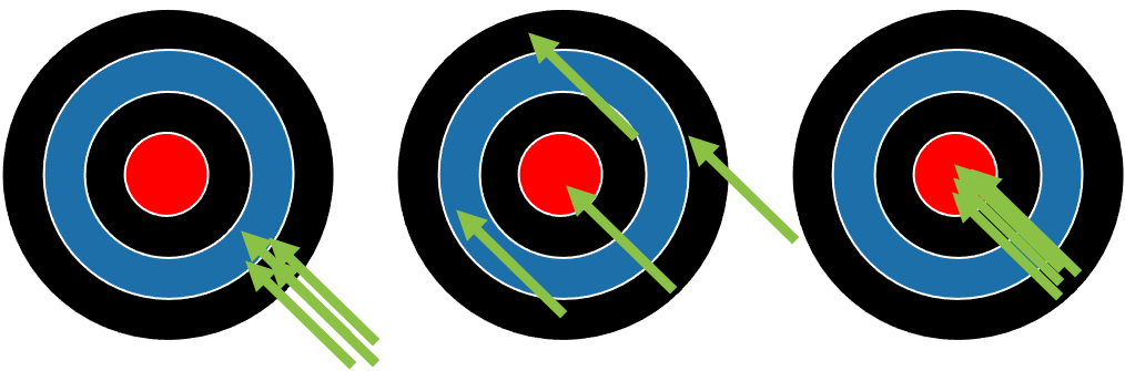
Let’s take a look at two examples to differentiate between reliability and validity. To be clear from the beginning, valid data must be reliable, but not all reliable data are valid. The first example is the classic example you will find in many statistics textbooks that comes from archery and is observed in Figure 6.1 below. There are 3 different targets and 3 archers. The first archer fires all their arrows and none of them hit the bullseye that they were aiming for, but they are pretty consistent in where they do hit the target. Since they do not hit the mark, they were aiming for, they cannot be considered valid. But, since they are consistent, they can be considered reliable. This means that we could actually be bad at something but be bad consistently and we’d be considered reliable. The word reliable in itself does not necessarily mean good. Let’s take a look at the second target. Here we see that the archer does hit the bullseye once but is pretty spread out with the rest of the arrows. They likely hit the bullseye once by chance alone and since the arrows are pretty spread out, we can’t say they are reliable. If they aren’t reliable, the aren’t valid either. On the 3rd target the archer hit the bullseye with every arrow. Since they consistently did this, they are reliable. Since they hit the mark they were going for, they are relevant and also valid.
Let’s look at an example where someone might confuse reliability and validity. There is currently at least one cell phone service provider that states that they are ”the most reliable network” and they market this as a reason you should switch to them. But should you? What does this actually mean? Being the most reliable doesn’t actually tell us anything of value and they may be depending on potential customers' confusion in this area. From a statistical standpoint, this marketing simply states that they are the most consistent carrier. They could be consistently good or consistently bad and could still be telling the truth. We don’t actually know from the information they provided. What customers are generally most concerned with (other than price) is whether or not they will have coverage in their area and this statement doesn’t provide any information on that aspect.
Reliability
Concerning reliability, objectivity is a specific type of reliability. It is also known as interrater reliability, which refers to the reliability between raters or judges.[1] Whenever we see the prefix “inter,” that refers to “between” and the prefix “intra” refers to “within.” An easy way to remember this is the difference between intercollegiate athletics (played between universities) and intramural athletics (played within the university). As an example of objectivity, consider an exam you take for a college course. Which of the following is likely more influenced by the grader, a multiple-choice exam, or an essay-based exam? The multiple-choice exam is more objective, less influenced, and the essay-based exam is more influenced or more subjective.
We would like to have most of our data be objective so that we aren’t introducing any bias, but sometimes we may not be able to avoid that. Can you think of an example? How about the RPE scale? The rating of perceived exertion can be used in many ways and is a cheap way to quantify the level of intensity of a given exercise. Unfortunately, it is highly subjective, and this can lead to issues when interpreting the values.
| Judge | Adelaide Byrd | Dave Moretti | Don Trella | |||||||||
|---|---|---|---|---|---|---|---|---|---|---|---|---|
| Fighter | Alvarez | Alvarez | Golovkin | Golovkin | Alvarez | Alvarez | Golovkin | Golovkin | Alvarez | Alvarez | Golovkin | Golovkin |
| Rd. | Rd. Score | Total Score | Rd. Score | Total Score | Rd. Score | Total Score | Rd. Score | Total Score | Rd. Score | Total Score | Rd. Score | Total Score |
| 1 | 10 | 9 | 10 | 9 | 10 | 9 | ||||||
| 2 | 10 | 20 | 9 | 18 | 10 | 20 | 9 | 18 | 10 | 20 | 9 | 18 |
| 3 | 10 | 30 | 9 | 27 | 9 | 29 | 10 | 28 | 9 | 29 | 10 | 28 |
| 4 | 9 | 39 | 10 | 37 | 9 | 38 | 10 | 38 | 9 | 38 | 10 | 38 |
| 5 | 10 | 49 | 9 | 46 | 9 | 47 | 10 | 48 | 9 | 47 | 10 | 48 |
| 6 | 10 | 59 | 9 | 55 | 9 | 56 | 10 | 58 | 9 | 56 | 10 | 58 |
| 7 | 9 | 68 | 10 | 65 | 9 | 65 | 10 | 68 | 10 | 66 | 9 | 67 |
| 8 | 10 | 78 | 9 | 74 | 9 | 74 | 10 | 78 | 9 | 75 | 10 | 77 |
| 9 | 10 | 88 | 9 | 83 | 9 | 83 | 10 | 88 | 9 | 84 | 10 | 87 |
| 10 | 10 | 98 | 9 | 92 | 10 | 93 | 9 | 97 | 10 | 94 | 9 | 96 |
| 11 | 10 | 108 | 9 | 101 | 10 | 103 | 9 | 106 | 10 | 104 | 9 | 105 |
| 12 | 10 | 118 | 9 | 110 | 10 | 113 | 9 | 115 | 10 | 114 | 9 | 114 |
| Final Score | 118 | <-Winner</td> | 110 | Final Score | 113 | Winner-> | 115 | Final Score | 114 | Draw | 114 | |
Table 6.1 depicts another example of objectivity and interrater reliability. Back in 2017, Canelo Alvarez and Gennady Golovkin fought to a split-decision draw. While you generally don’t want any fight to end in a draw, this one was much worse when you examine the score cards. The scorecards were transcribed into a table here from each of the 3 judges. If you are not familiar, both boxing and MMA use a 10/9 ”must” scoring system where whomever wins the round gets 10 points and the other fighter gets 9 points. If the round was particularly lopsided, a score of 8 may be awarded to the loser instead of 9, but that is quite rare. So, you can see how each judge scored each round and then totaled these scores to determine the overall winner. What was interesting was how differently Adelaide Byrd scored this fight from both Dave Moretti and Don Trella . She scored the fight as a convincing victory for Alvarez (Alvarez 118 to Golovkin's 110), while Moretti and Trella scored the fight much closer (113 to 115 and 114 to 114). There was a lot of blowback after this fight when the scorecards were released, and Byrd was actually suspended for some time. Based on the consistency between the other two judges, we might say that Byrd is not a reliable judge or more specifically, she does not seem to be as objective and lacks interrater reliability.
Relative and Absolute Measures of Reliability
Many of the variables we measure in exercise and sport science can be used to produce relative and absolute values. Consider oxygen consumption (VO2), strength, and power measurements. Each can be used to produce a measure relative to the subject's body mass (ml/kg/min, N/kg, or W/kg, respectively) or an absolute measure (l/min, N, W, respectively). Similarly, reliability can be measured relatively or absolutely. Relative measures of reliability are slightly different in their usage as they measure reliability relative to a specific sample or population. Relative measures of reliability provided an error estimate that differentiates between the subjects in a sample. As a result, these findings should not be applied to any sample or population that is different than the one studied. For example, imagine you are using a bioelectical impedance analysis (BIA) unit to quantify body composition for a study. Previous research has published reliability findings on the exact same device that you will be using. You could save a lot of time by simply citing the previous research demonstrating its reliability instead of completing your own analysis. Unfortunately, if relative measures of reliability were used (or those are the measures you wish to discuss), those findings are specific to the sample tested. This means that variable reliability should be evaluated with each new study or each new sample/population being tested if/when relative measures of reliability are used. This also means that comparisons of relative reliability findings should not be completed when the samples/populations are not similar. Absolute measures of reliability provide an estimate of the magnitude of the measurement error. Absolute measures of reliability can be inferred across samples as long as they have similar characteristics. When evaluating reliability, both relative and absolute measures of reliability should be included. Please refer to Figure 6.xxx below that provides options for evaluating each.
Evaluating Reliability
We might understand reliability a little better when we consider the observed, true, and error scores. As we have seen before, the observed score is the sum of the true score and error score.[2] In theory, the true score exists, but we will never be able to measure it. Anything that causes the observed score to deviate from the true score can be considered error.
If we are essentially attempting to calculate how a variable measure might change from trial to trial we could consider it from a variance perspective. Or more specifically, a "variance unaccounted for" perspective which we discussed in the chapter on correlation. If one trial can predict a very large amount of the variance in another trial, this information is useful in terms of reliability as we will also know how much error variance there is from one trial to the next. Many methods to evaluate reliability are based off of the correlation and similar to the PPM correlation, scores can range from 0 to 1. It is generally desired that reliability coefficients be greater than 0.8.
Test-Retest reliability
The example described above is one version of test-retest reliability where one trial of a measure is evaluated against another. If the data is reliable, it should produce similar values. When using a PPM correlation to evaluate this, it is sometimes referred to as an "interclass" correlation coefficient. The prefix "inter" is used with a PPM coefficient because it is most often used to evaluate correlations "between" 2 variables. The term "intraclass" correlation coefficient (ICC) is likely more correct here as we are actually evaluating the same variable "within" multiple trials. As you may have noticed, this differentiation between inter- and intra- here can become a little confusing and is mostly semantic and/or simply used to classify different types of tests. As such, you may see the abbreviation ICC used for both. Either way, they are both considered relative measures of reliability.
| Subject | Trial 1 | Trial 2 |
|---|---|---|
| 1 | 0.33 | 0.35 |
| 2 | 0.39 | 0.41 |
| 3 | 0.25 | 0.31 |
| 4 | 0.44 | 0.44 |
| 5 | 0.35 | 0.32 |
| 6 | 0.34 | 0.31 |
| 7 | 0.22 | 0.24 |
| 8 | 0.33 | 0.33 |
| 9 | 0.31 | 0.26 |
| 10 | 0.44 | 0.48 |
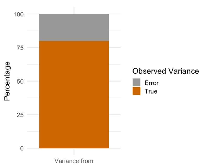
We can use Dataset 6.1 and/or the data in Table 6.2 above to evaluate the test-retest reliability of jump heights across 2 trials with a PPM correlation. Running a simple correlation we find a r value of 0.897. This means that we can predict 80.4% of the variance in trial 2 with the data from trial 1 (using the coefficient of determination (r2)). Or we could subtract that value from 100% and say that the error variance is 19.6%.
The above example assumes the trial data was collected one right after the other in the same session. If a significant amount of time has passed between measurements, the term stability should be used instead of reliability. Stability is used to determine how subjects hold their scores.
Chronbach's Alpha (ICCa)
The intraclass correlation Chronbach’s Alpha coefficient or ICCa is one of the most commonly used intraclass correlation models. It examines variance from 3 different components: subject variance, trial variance, and subject-by-trial variance.
Most statistical software will have a function to calculate this. MS Excel does not, but as you can see by the formula, it can calculated with other Excel functions, which we've already learned how to calculate. We’d just need to calculate the variance for each of the components mentioned previously (trial, the variance for all trials, and the sum of each trial’s variance). Then we could plug that data into the formula below, where [asciimath]alpha[/asciimath] = alpha, [asciimath]k[/asciimath] = number of trials, [asciimath]sum_(i=1)^{k}[/asciimath] = sum of each trial's variance, [asciimath]sigma_(yi)^{2}[/asciimath] = variance from trial [asciimath]i[/asciimath], and [asciimath]sigma_x^{2}[/asciimath] = total variance.
[asciimath]alpha = (k/(k-1))*(1-(sum_(i=1)^{k}sigma_(yi)^{2})/sigma_x^{2})[/asciimath]
While calculating alpha is possible in MS Excel, it isn't exactly quick or easy and many used other statistical programs as a result.
The ICC is considered a relative measure of reliability, which means that it is specific to your sample. As mentioned earlier, you cannot infer the reliability found during testing from one sample to another if the ICC was the measure used.
Calculating Chronbach's Alpha (ICCa) in JASP
In order to calculate Chronbach's [asciimath]alpha[/asciimath] in JASP, each trial will need to be included as it's own column and a minimum of 3 trials is required. As of JASP version 0.14.1, 3 trials were required, but previously (and potentially future versions) JASP users have been able to calculate ICCa with 2 trials. This is important as getting 3 maximal effort trials for performance data isn't always realistic.
This dataset includes 3 trials of jump height data measured in meters. Once the data have been imported, click on the Reliability module drop-down arrow and select the Classical version of the Single-Test Reliability Analysis. Then move each trial over to the Variables box and scroll down to the Single-Test Reliability menu. Deselect McDonald's ω and select Chronbach's α. The results should now appear.
|
Frequentist Scale Reliability Statistics |
|||
|---|---|---|---|
| Estimate | Cronbach's α | ||
| Point estimate | 0.981 | ||
| 95% CI lower bound | 0.928 | ||
| 95% CI upper bound | 0.996 | ||
A Chronbach's α value of 0.981 is quite good as it is very close to 1. The 95% confidence intervals (CI) are also included. They indicate the 95% likelihood range where we would find the result if tested again with the same sample. This result could be written as ICCa = 0.981 [0.928,0.996], which is inidcating the ICCa 95% CI range from 0.928 to 0.996.
Issues with Correlational Methods
One issue with using a PPM correlation to evaluate reliability is that it is bivariate in nature and therefore can only evaluate 2 trials. Other methods like Chronbach's Alpha (described above) or those based on a repeated measures ANOVA can overcome this issue.
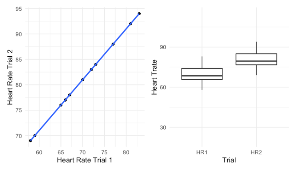
Another issue that impacts all correlational reliability models (including ICCa above) happens when there is a consistent difference between trials. Table 6.2 shows a dataset containing 2 trials of heart rate data that correlates perfectly (r = 1.00), but is statistically different.
| Subject | HR trial 1 | HR trial 2 |
|---|---|---|
| 1 | 66 | 77 |
| 2 | 67 | 78 |
| 3 | 81 | 92 |
| 4 | 73 | 84 |
| 5 | 59 | 70 |
| 6 | 65 | 76 |
| 7 | 83 | 94 |
| 8 | 77 | 88 |
| 9 | 72 | 83 |
| 10 | 70 | 81 |
| 11 | 58 | 69 |
| 12 | 66 | 77 |
If a PPM correlation is run on this data a perfect 1.0 correlation is observed and you can see this in the scatter plot below in Figure 6.3 with a perfectly straight trendline. So, is this data reliable? Nope. In fact, a paired samples t test reveals a p value of less than 0.000 indicating the trials are statistically different. Hopefully you examined the data and noticed a pattern. Each value in trial 2 is exactly 11 beats per minute higher than that of trial 1. The mean bpm of trial 1 is 69.75, while the mean of trial 2 is 80.75. Clearly, there is a difference and this can be seen in the box plot also in Figure 6.3. But why does our correlation not pick up on this? It’s because there is a consistent difference in the values. Think about a correlation as a ranking within the group. If you rank each subject according to their HR, what will happen to their rank if we change each trial #1 value by the same amount. Their rank will be unaffected. So, they still vary the same way, which means the correlation will not recognize it.
Equivalence Reliability for Exams or Questionnaires
Often with exams or questionnaires, one might want to use multiple forms of the instrument. In order to evaluate their equivalence, each subject must participated in each exam. Again, the PPM could be used to determine how well the scores on one exam correlate with the other. If the r value is high enough, they might be considered equivalent.
While the equivalence method may be used for exams and questionnaires, it is generally not recommended to use different forms of data collection as substitutes for one another. This is especially true for performance testing as we've seen in one of the issues with using correlation as a measure of reliability above. Variables or trials that change similarly may look strongly correlated or reliable, but the magnitudes may be different. So whichever tool is used initially may not be interchangeable with another one.
One issue with the equivalence method is that it may be difficult to find subjects to take an exam once, let alone on 2 separate occasions. Another alternative is to administer one exam, but split the test in half afterward to evaluate the equivalence of the 2 halves to be used later. This is referred to as split-halves reliability.
Another issue with administering questionnaires is the length of the questionnaire. You are much more likely to get subjects to complete the questionnaire if it is short. That being said. the easiest way to increase the reliability of a questionnaire is to make it longer. Ideally, your questionnaire would be long enough to be reliable, but short enough that subjects do not quit while doing it. Finding this optimal zone could end up being somewhat of a "guess and check" method. Fortunately, there is a way to predict how the reliability might change depending on how we change the length of the exam or questionnaire (increasing or decreasing) called the Spearman-Brown Prophecy Formula.[3]
[asciimath]r_"kk" = (k*r_11)/(1+r_11*(k-1))[/asciimath]
rkk = predicted reliability coefficient, k = # of times the length of the test has changed, and r11 = the original reliability coefficient
Imagine an exam was given that had a length of 25 items and its reliability was previously evaluated as 0.555. If we cahnge the length to 50 items, we are doubling its length. So, k = 2. What would the new predicted reliability be then? This can be predicted if the values are plugged into the formula.
[asciimath]r_"kk" = (2*0.555)/(1+0.555*(2-1))[/asciimath]
[asciimath]r_"kk" = 1.11/1.555[/asciimath]
[asciimath]r_"kk" = 0.714[/asciimath]
Doubling the length of the exam increased the reliability coefficient (predicted) to 0.714, which is going in the direction desired. What do you think would happen if we instead shortened the original 25 item test length to 15 items? We can find k by dividing 15 by 25. This gives us a k of 0.6. Since the k is now less than 1, we will be decreasing the value of the numerator. If the value of the denominator stays the same, the value will have to decrease. Decreasing the item length to 15 shrinks the rkk to a value of 0.214.
Standard Error of Measurement (SEM)
The standard error of the measurement or SEM is an absolute measure of reliability, meaning that it indicates the magnitude of the measurement error and you can infer reliability results from one sample to another assuming they have similar characteristics. It essentially tells us how much the observed score varies due to measurement errors. An added benefit of this measure is that it stays in the units of the original measure. So, if we were measuring VO2max in ml/kg/min, the SEM value would also be in ml/kg/min. We can calculate the SEM as the standard deviation (σ) times the square root of 1 minus the ICC value. Some statistical software will have a function for this measure, but not all. So it is pretty common that you may need to calculate this one by hand.
[asciimath]SEM=sigma*sqrt(1-I C C )[/asciimath]
Consider an example where we have a mean of 44.1 ml/kg/min, a standard deviation of 12.6 ml/kg/min, and an ICC of 0.854, what is the SEM? All the information needed is provided, so we can just plug the information in to determine it and we end up with a value of 4.81 ml/kg/min. So, is that good or bad? We can interpret the SEM by it’s size relative to the mean. 4.81 is roughly 11% of 44.1 (4.81/44.1*100=10.9%). We generally want our values to be pretty low here, but there is no strict cutoff.
One final note on the SEM is that it assumes that your data are homoscedastic, meaning that there is no proportional bias. If the portion of your data that are either really large or really small and have a greater chance to be an error than the portion in the middle, it would not be considered homoscedastic. It would then be considered heteroscedastic (proportional bias is present). This assumption should be checked prior to using the SEM. If your data violate this assumption, you can use the coefficient of variation, which we will discuss next. The assumption of homoscedasticity can be checked with several statistical test depending on your data type and the models used. The most common are the Levene's test of homogeneity (for samples with multiple groups) or the Breusch-Pagan test (without groups).
Calculating the SEM in JASP
JASP does not have a simple check box to add in the SEM to reliability analysis, but you can simply add the mean and standard deviation to the tabular results shown earlier by checking boxes.
|
Frequentist Scale Reliability Statistics |
|||||||
|---|---|---|---|---|---|---|---|
| Estimate | Cronbach's α | mean | sd | ||||
| Point estimate | 0.981 | 0.344 | 0.004 | ||||
| 95% CI lower bound | 0.928 | ||||||
| 95% CI upper bound | 0.996 | ||||||
Now the SEM can be calculated.
[asciimath]SEM=0.004*sqrt(1-0.981)[/asciimath]
This produces an SEM of 0.0006 m, which is very small. Don't forget that the SEM will carry the same unit of measure as the original variable.
Coefficient of Variation (CV)
Unlike the SEM, the coefficient of variation, or CV, assumes that your data does show proportional bias (heteroscedastic). Much of the data we see in sport and human performance are this way.[4][5] Those that can produce a lot of force or those that can run really fast are more prone to have errors in their measurements. This has nothing to do with the subjects themselves, but when we test those that will produce some of the more extreme values our equipment is more likely to produce an error. The CV is more appropriate for this type of data. It’s also much easier to calculate since we only need to know the mean and standard deviation of the sample. We simply divide the standard deviation (σ) by the mean ([asciimath]m[/asciimath] and multiply by 100.
[asciimath]CV=(sigma/m)*100[/asciimath]
This gives us a percentage that will tell us how much variation there is about the mean of the sample. In general, we want this value to be less than 15%. Unfortunately, most statistical software does not include functions to calculate this and that may be because it is pretty simple to do ourselves. So you will most often need to compute this one yourself.
Let’s revisit our VO2max example. With a mean of 44.1 and a standard deviation of 12.6, what is the CV? 12.6 divided by 44.1 is 0.2839. We multiply that by 100 and we are left with a CV of 28.39%.
[asciimath]CV=(12.6/44.1)*100=28.39%[/asciimath]
This is above our desired 15% cutoff, so this does show a decent amount of variation. Hopefully you are also now noticing that we had a decent ICC value of 0.854, but a poor CV value. These are both reliability measures, so do we have both good an bad reliability? Actually, that is somewhat true. Keep in mind that the ICC is a relative measure of reliability and the CV and the SEM are absolute measures of reliability. So we could say that our VO2max data shows good relative reliability, but less than desirable absolute reliability.
Reliability versus Agreement
The way we defined reliability earlier is accurate, but is also somewhat broad, which leads to some confusion about the difference between reliability and agreement from a statistical perspective. This is generally just semantics, but I will try to clear it up a little bit here before we discuss quantifying agreement. Both are concerned with error, but reliability is more concerned with how that error relates to each person’s score variation and agreement is concerned with how closely the scores bunch together.[6]
If we move from the theoretical definition to the practical usage of these two, we see a greater divide generally. Agreement in kinesiology studies is almost exclusively used when working with dichotomous data such as, win or lose, pass or fail, or left or right. Reliability assessments like we discussed previously are used on other types of data. Methods of measuring agreement also differ in that they can be used with validity measures as well.
Now that we have discussed these differences, let’s take a look at how we can evaluate agreement with the proportion of agreement and the Kappa coefficient.
Proportion of Agreement (P)
Our first measurement of dichotomous agreement is the proportion of agreement. It is the ratio of scores that agree to the total number of scores. Looking at the diagram in Figure 6.4 below, that you may recognize as a chi square contingency table. Each inner quadrant is named as n and either 1, 2, 3, or 4. Quadrants n1 and n4 represent the number of scores that agreed between trials, days, or tests and quadrant n2 and n3 represent the disagreements. For example, let’s say we are classifying strength asymmetry of the lower body. If a subject has demonstrated to have a left-side asymmetry in trial 1 and a left-side asymmetry in trial 2, they would be counted in the top left quadrant (n1), where we see that 21 subjects were counted. If they presented with a right-side asymmetry in trial 1, but a left-side asymmetry in trial 2, they would be counted in the top right or n2 quadrant and this square represents a disagreement between trials. Likewise, n3 also represents a disagreement. Subjects counted there present with a left-side asymmetry in trial 1 and a right-side asymmetry in trial 2. Finally, n4 represents those who present with right-side asymmetries in both trials, so it is our other agreement quadrant.

In order to calculate the proportion of agreement, we simply divide the total number of agreements (found in n1 and n4) by the total number of scores (summing all quadrants).
[asciimath]P=(n_1+n_4)/(n_1+n_2+n_3+n_4)[/asciimath]
[asciimath]P=(21+19)/(21+11+13+19)[/asciimath]
[asciimath]P=(40/64)=0.625[/asciimath]
This leaves us with 40 agreements out of 64 scores or a proportion of agreement of 0.625. We can convert this to a percentage of agreement by multiplying by 100. This would mean that we have 62.5% agreement between trial 1 and trial 2. The proportion of agreement ranges from 0 to 1 where higher values indicate more agreement
One issue with this method is that it does not account for chance occurrences, which we have seen can cause issues in our results and interpretations.
Kappa coefficient (K)
The Cohen’s Kappa coefficient, or simply Kappa coefficient does account for agreements coming from chance alone. This makes it a more frequently used method. Although, since you must calculate the proportion of agreement as part of Kappa, you could argue that it is used just as frequently.
To calculate Kappa, you must first calculate the proportion of agreement as we did previously. We then subtract the proportion of agreement coming from chance and divide that value by one minus the proportion due to chance. We will discuss how to calculate the proportion due to chance on the upcoming slides.
[asciimath]K=((P-P_c)/(1-P_C))[/asciimath]
Kappa values may range from -1 to +1, similar to correlation values, but we generally only want to see positive values here. Negative values indicate that we have more observed agreements coming due to chance occurrences. Similar to correlations, values closer to 1 indicate greater agreement. You can see the interpretation scale created by Landis and Koch (1977) below.[7]
| K Range | Interpretation |
|---|---|
| < 0 | less than chance agreement |
| 0.01 to 0.20 | slight agreement |
| 0.21 to 0.4 | fair agreement |
| 0.41 to 0.6 | moderate agreement |
| 0.6 to 0.8 | substantial agreement |
| 0.81 to 0.99 | almost perfect agreement |
Kappa is the preferred method for evaluating agreement since it does account for chance; however, due to the way proportion due to chance is calculated, smaller sample studies are not ideal candidates for this method.
Moving forward with calculating the Kappa coefficient, it makes sense to format the data into a true table like the one in Table 6.7. This is the same data from before, but now the sums of the columns and rows have been added (Total).
| Trial 1 | ||||
|---|---|---|---|---|
| Trial 2 | Left | Right | Total | |
| Left | 21 | 11 | 32 | |
| Right | 13 | 19 | 32 | |
| Total | 34 | 30 | 64 | |
In order to calculate the proportion of agreement due to chance (Pc), we must add in marginal data which are the sums of the rows and columns. Those values are then multiplied and then divided by the total n2. This must be done for row 1/column 1 and for row 2/column 2, so we will end up with 2 values for Pc. They can then be added to calculate the total Pc. In this case, row 1 has a marginal value of 32 and column 1 has a marginal value of 34. Row 2 has a marginal value of 32 and column 2 has a marginal value of 30. The total n should be the same as the sample size, 64.
[asciimath]P_c=(32*34)/64^2=0.27[/asciimath]
and
[asciimath]P_c=(32*30)/64^2=0.23[/asciimath]
These can be added together to produce the total Pc needed to calculate Kappa.
[asciimath]P_c=0.27+0.23=0.50[/asciimath]
This value can now be used to calculate Kappa using the formula previously shown.
[asciimath]K=(0.625-0.5)/(1-0.5)=0.25[/asciimath]
What do you notice? The Kappa value is quite a bit lower than the proportion of agreement. Why do you think it decreased? It decreased because it factored out the proportion of agreement that was coming from chance occurrence.
There is nothing special about completing this analysis in MS Excel. Assuming the table is set up correctly, the summation column and rows can be added simply along with the other calculations. If one does this sort of analysis frequently, it might be worthwhile to set up a template file so that the calculations can be completed as soon as the new values are typed in. As of JASP 0.14.1, there is not a current solution for calculating Kappa, but this could change with future versions.
Validity
As mentioned previously, validity refers to how truthful a measure is. That is a somewhat broad definition as validity can take on many forms. There are 3 main forms of validity: content-related reliability, criterion-related reliability, and construct-related reliability.
Content-Related Validity
Content related validity is also known as "face validity" or logical validity. It answers the question does the measure clearly involve the performance to be evaluated. Generally, there isn't any statistical evidence required to back this up. For example, if it rains and I don't have an umbrella, I will get wet walking outside. If it is raining on a Monday and I forgot my umbrella, what will happen?
Evaluations of content validity are often necessary in survey-based research. Surveys must be validated before they can be used in research. This is accomplished by sending a draft of the survey to a content expert who will evaluate if the survey will answer the questions the experimenters are intending them to.
Criterion-Related Validity
Criterion-related validity attempts to evaluate the presence of a relationship between the standard measure and another measure. There are two types of criterion-related validity.
- Concurrent validity evaluates how a new or alternative test measures up to the criterion or "gold standard" method of measurement.
- Predictive validity evaluates how a measurement may predict the change or response in a different variable.
Concurrent validity is pretty common in technology related kinesiology studies. Think about a new smartwatch that counts repetitions, measures heart rate, heart rate variability, and tracks sleep. A single study could seek to validate one or more of these measures, but this example will focus on heart rate and heart rate variability. What would the gold standard method of measuring these likely be? Probably an EKG. So a researcher could concurrently (or simultaneously) measure those variables with the new smartwatch and an EKG in 50 subjects. The validity of the smartwatch would be dependent on how well it measures up to the gold standard measure, the EKG. If the values are very different, we'd likely conclude that it isn't valid. As a side note, it is also common to evaluate reliability during these types of studies.
Click here to see an example of one of these types of studies that was presented as a poster.
Predictive validity seeks to determine how variation in specific variables might predict outcomes of other variables. A good example of this is how diet, physical activity, hypertension, and family history can be predictive of heart disease. Regression has been discussed in this book before, and hopefully you recall that the prediction equation will predict values or outcomes based upon specific variable inputs. Those prediction values are usually not perfect, and the discrepancy between the predicted values and the true values is known as the residual. The larger the residual values are, the less predictive validity we observe.
A key aspect of criterion-related validity is determining what the criterion measure should be. Keep in mind that predictive validity uses past events and data to create prediciton equations. If it is the goal to prevent some sort of performance, it would be a good idea to validate the predicitions against the actual performance whenever that happens (though this may not always be possible). For concurrent validity, it is always best to use the gold standard test as the criterion. When that is not possible, another previously validated test may be used instead.
Construct-Related Validity
Construct-related validity evaluates how much a measure can evaluate a hypothetical construct. This often happens when one attempts to relate behaviors to test scores or group membership. We often see this with political parties and polling results. Members of one party often vote a specific way on certain topics, while the other party would usually vote the opposite way.
These constructs are easy to imagine, but often difficult to observe. Consider a hypothetical example involving ethics in sport. How can you determine which athletes are cheaters and which play fair? This isn't easy because they don't wear name tags describing as much. But, you probably have some thoughts about specific athletes in your favorite sport. You might really like some and really dislike others based on past events observed.
Studying this type of research question is quite difficult too. You might come up with scenarios that put subjects into situations where they are forced to make several choices and depending on the test results, you classify them as a "good sport" or a "bad sport" based on the number of times they chose to break the rules. Once they are classified with a grouping variable, many of the means comparison test methods like a t test or an ANOVA could then be applied.
Evaluating Validity
By now, you should be recognizing just how useful the correlation can be. It will be the primary method for validation as well. If you are keeping track, it can be used to evaluate test-retest reliability, objectivity, equivalence reliability and both concurrent and predictive validity. That's in addition to everything discussed in the chapter on correlation. At this point if you had to guess which statistical test should be run for a given example, the correlation most likely has the highest probability of being correct. As correlation in both MS Excel and JASP have already been demonstrated, they will not be shown again. Please refer to Chapter 3 if you need to review.
Similar issue with correlation (valid does not mean interchangeable)
While we will nearly always select the correlation for our statistical evaluation of validity, there is one caveat. If a device is highly correlated with the gold standard or criterion measure, we will likely conclude that it is valid. But, that does not mean that we can use the two devices interchangeably. If you read the research poster example above, you’ve seen why. In that study multiple vertical jump assessment devices were validated concurrently. Most were highly correlated with the criterion measure (a force plate), but t tests also revealed that they were statistically different. Stating that devices can be highly related but different may sound counterintuitive, but this comes back to the concept we discussed earlier in this chapter on consistent change. If one of the devices consistently gives an inflated value, but gives everyone that same inflated value, the correlation will still be very strong. A comparison of the means will likely show the difference though. So, the moral is that even though both devices may be valid, you should stick with the same one throughout your study because they can still be different. Please refer back to Figure 6.3 for a visual representation of this issue.
Bland-Altman assessment of agreement
Building on the issue with consistent differences just discussed, a different technique that evaluates agreement was created by Bland and Altman in 1986. If you recall, from the reliability portion of this chapter, many also use agreement when evaluating reliability.[8] This method will be described along with a practical example.
| Gold Standard | Smartphone |
|---|---|
| 63 | 64 |
| 77 | 75 |
| 76 | 80 |
| 83 | 85 |
| 107 | 117 |
| 85 | 85 |
| 111 | 87 |
| 86 | 90 |
| 93 | 113 |
| 105 | 105 |
| 89 | 98 |
In Table 6.7 and dataset 6.4 (click here to download dataset 6.4) we have a new smartphone app that uses the camera’s led flash to measure heart rate. This will be validated against an EKG as the criterion measure. The new smartphone app correlates pretty well with it, with an r value of 0.761. It isn’t perfect, but that is pretty strong as it accounts for roughly 58% of the variance (r2 = 0.580).
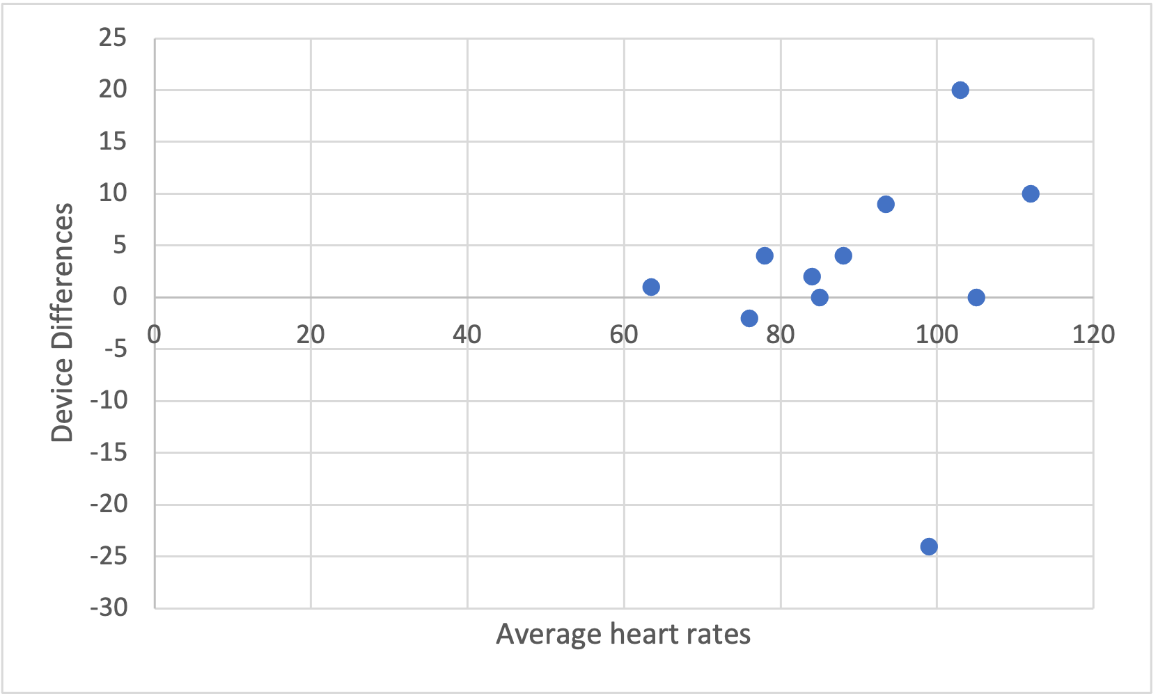
One issue that Bland and Altman brought up is that the measure magnitude may influence the accuracy of the measurement in some data. This has actually already been discussed earlier in this chapter as proportional bias. If our larger or smaller values from the smartphone deviate more than the middle values from the gold standard, we would likely have some proportional bias or heteroscedasticity. We can examine this with a plot by adding in the measure differences and plotting those against the averages.
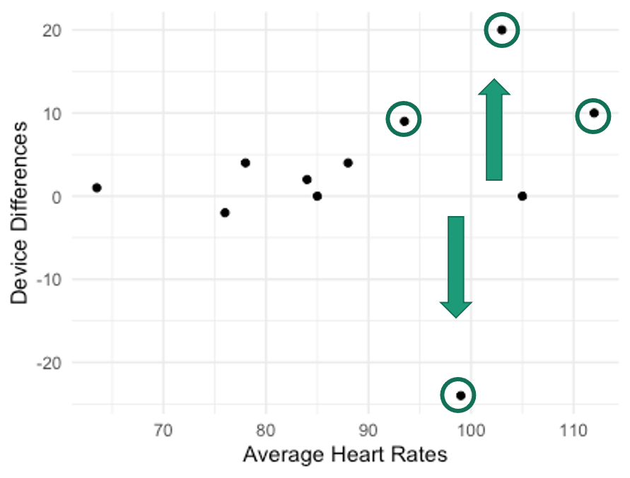
Notice in Figure 6.5 several of the higher heart rate values deviate further from the horizontal 0 line. This demonstrates a trend where the higher the heart rate value is the larger the error magnitude compared to the EKG. In order to create this plot, we will need to compute a couple of new columns for our dataset.
| Gold Standard | Smartphone | mean | difference |
|---|---|---|---|
| 63 | 64 | 63.5 | 1 |
| 77 | 75 | 76 | -2 |
| 76 | 80 | 78 | 4 |
| 83 | 85 | 84 | 2 |
| 107 | 117 | 112 | 10 |
| 85 | 85 | 85 | 0 |
| 111 | 87 | 99 | -24 |
| 86 | 90 | 88 | 4 |
| 93 | 113 | 103 | 20 |
| 105 | 105 | 105 | 0 |
| 89 | 98 | 93.5 | 9 |
Now we've added in another column depicting the differences between each of the smartphone and the EKG heart rate measurements and another one that averaged the EKG and smartphone values. This data was used in Figure 6.5, which shows the device differences on the y axis and the averages on the x axis. This funnel type shape is indicative of heteroscedasticity no matter which direction it is pointing. Given what is seen here, it seems that whenever higher heart rates are collected, there is more difference from the EKG than when lower heart rates are collected. This should be a cause for concern if one wishes to used this for measurement during exercise when higher heart rates should be expected. The validity will suffer in this case.
Creating a Bland-Altman Plot in MS Excel
Beginning with Dataset 6.4, the final 2 columns appearing in Table 6.8 need to be added before the Bland-Altman plot can be created. Creating the mean column can be accomplished with the =AVERAGE() built-in Excel function where both heart rate values for a given row are included. Copying and pasting this value for each row will produce values for each. [9] The differences column can be computed by creating a differences column which subtracts the EKG value from the Smartphone value. This can be calculated in Excel as B2-A2 in Dataset 6.4. Copying and pasting the formula all the way down will produce values for each of the rows. Next, the average between the EKG heart.
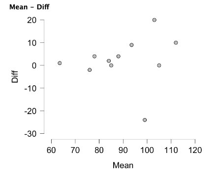
Now highlight the two new columns and select Insert from the ribbon. Selecting the basic scatter plot should produce a plot that looks very simlar to the one shown below in Figure 6.6. It will not be identical because Figure 6.5 was created with R and the x axis has been adjusted to zoom in on the data. Formatting the x axis in Excel may also be completed. Adding chart elements such as axis titles are also very helpful for viewers.
Creating a Bland-Altman Plot in JASP
Similar to the solution in Excel, the final 2 columns need to be created. But, you first must make sure that the imported data have the correct variable types selected. More than likely, the SmartPhone data was imported as ordinal. This will be an issue if it is not changed to scale. If you recall back to Chapter 2 of this book, only scale data can be manipulated and the result be useful. If we try to compute the column while it is still listed as ordinal, it will remain blank.
The mean of the EKG and smartphone measures can be created by adding the two variables together and dividing by 2.[10] The difference column can be created by subtracting the EKG value from the smartphone value. Both of these are considered computed variables, so they must added by clicking the plus sign to add a new variable. As you may recall, variables can be computed using JASP's drag and drop formula builder or using R syntax. Use whichever you are comfortable with, but don't be afraid of R here as it is very straightforward in this example. Using the R syntax to compute the mean you would need to type in "(EKG+SmartPhone)/2" and the difference column would be "Smartphone-EKG." Then click compute and the new columns should be populated with data.
The Bland-Altman plot can be created in the Descriptives module of JASP. After clicking the Descriptives icon, move the two newly created variables into the variables box. Now move down to the Plots menu and check the Scatter Plots option. Your plot will now be created, but you'll need to make a few adjustments to make it look similar to Figure 6.5. By default, density plots are included above and to the right of the scatter plot. Check none to remove both of those. Now click to uncheck and remove the regression line and the plot should look very similar to Figure 6.7 below. If it looks like the same plot but rotated 90°, you likely have the variables listed out of order. Mean (or the gold standard) should be listed prior to the difference variable. To fix this, simply remove the variable listed first in the Variables box and add it again so that it appears afterward.
Closing remarks
As the chapter name indicates, reliability and validity are both very important. That being said, if we also understand objectivity, relevance, and agreement, we will likely have a better understanding of reliability and validity. While many may incorrectly do this, the results of reliability and validity analyses are difficult to generalize. This is because the studies where they were analyzed often utilizes different sample characteristics than those they (or you) want to generalize to. Even when you have a similar population, you may not be able to standardize a lot of other variables, so you probably shouldn’t expect as favorable of outcomes as have been published previously in a highly standardized laboratory study. But, if you follow the testing protocol as closely as possible, your results will be as reliable and valid as potentially possible.
- Morrow, J., Mood, D., Disch, J., and Kang, M. (2016). Measurement and Evaluation in Human Performance. Human Kinetics. Champaign, IL. ↵
- Vincent, W., Weir, J. 2012. Statistics in Kinesiology. 4th ed. Human Kinetics, Champaign, IL. ↵
- Morrow, J., Mood, D., Disch, J., and Kang, M. 2016. Measurement and Evaluation in Human Performance. Human Kinetics. Champaign, IL. ↵
- Bailey, C. (2019). Longitudinal Monitoring of Athletes: Statistical Issues and Best Practices. J Sci Sport Exerc.1:217-227. ↵
- Bailey, CA, McInnis, TC, Batcher, JJ. (2016). Bat swing mechanical analysis with an inertial measurement unit: reliability and implications for athlete monitoring. Trainology, 5(2):42. ↵
- de Vet HC, Terwee CB, Knol DL, Bouter LM. When to use agreement versus reliability measures. J Clin Epidemiol. 2006 Oct;59(10):1033-9. ↵
- Landis, JR and Koch, GG (1977). The measurement of observer agreement for categorical data. Biometrics, 33:159-174. ↵
- Bland JM, Altman DG. (1986). Statistical methods for assessing agreement between two methods of clinical measurement. Lancet;1(8476):307-10. ↵
- Note: that some may wish to use the gold standard value instead of the mean here. If using a Bland-Altman plot for reliability purposes (trial to trial agreement), the mean is necessary. If using if for validity purposes, it may not be, but this needs to be described and justified no matter which method is used. ↵
- Note: that some may wish to use the gold standard value instead of the mean here. If using a Bland-Altman plot for reliability purposes (trial to trial agreement), the mean is necessary. If using if for validity purposes, it may not be, but this needs to be described and justified no matter which method is used. ↵
refers to the consistency of data. Often includes various types: test-retest (across time), between raters (interrater), within rater (intrarater), or internal consistency (across items).
how well scores represent the variable they are supposed to; or how well the measurement measures what it is supposed to.
Relative measures of reliability provided an error estimate that differentiates between the subjects in a sample
Absolute measures of reliability provides an estimate of the magnitude of the measurement error.
