5 Chapter 5: Experimental and Quasi-Experimental Designs

In This Chapter You Will Learn

The four components of experimental and quasi-experimental research designs and their function in answering a research question

The differences between experimental and quasi-experimental designs

The importance of randomization in an experimental design

The types of questions that can be answered with an experimental or quasi-experimental research design

About the three factors required for a causal relationship

That a relationship between two or more variables may appear causal, but may in fact be spurious, or explained by another factor

That experimental designs are relatively rare in criminal justice and why

About common threats to internal validity or alternative explanations to what may appear to be a causal relationship between variables

Why experimental designs are superior to quasi-experimental designs for eliminating or reducing the potential of alternative explanations

Introduction

The teen court evaluation that began this chapter is an example of an experimental design. The researchers of the study wanted to determine whether teen court was more effective at reducing recidivism and improving attitudes compared to regular juvenile justice case processing. In short, the researchers were interested in the relationship between variables—the relationship of teen court to future delinquency and other outcomes. When researchers are interested in whether a program, policy, practice, treatment, or other intervention impacts some outcome, they often utilize a specific type of research method/design called experimental design. Although there are many types of experimental designs, the foundation for all of them is the classic experimental design. This research design, and some typical variations of this experimental design, are the focus of this chapter.

Although the classic experiment may be appropriate to answer a particular research question, there are barriers that may prevent researchers from using this or another type of experimental design. In these situations, researchers may turn to quasi-experimental designs. Quasi-experiments include a group of research designs that are missing a key element found in the classic experiment and other experimental designs (hence the term “quasi” experiment). Despite this missing part, quasi-experiments are similar in structure to experimental designs and are used to answer similar types of research questions. This chapter will also focus on quasi-experiments and how they are similar to and different from experimental designs.

Uncovering the relationship between variables, such as the impact of teen court on future delinquency, is important in criminal justice and criminology, just as it is in other scientific disciplines such as education, biology, and medicine. Indeed, whereas criminal justice researchers may be interested in whether a teen court reduces recidivism or improves attitudes, medical field researchers may be concerned with whether a new drug reduces cholesterol, or an education researcher may be focused on whether a new teaching style leads to greater academic gains. Across these disciplines and topics of interest, the experimental design is appropriate. In fact, experimental designs are used in all scientific disciplines; the only thing that changes is the topic. Specific to criminal justice, below is a brief sampling of the types of questions that can be addressed using an experimental design:

Does participation in a correctional boot camp reduce recidivism?

What is the impact of an in-cell integration policy on inmate-on-inmate assaults in prisons?

Does police officer presence in schools reduce bullying?

Do inmates who participate in faith-based programming while in prison have a lower recidivism rate upon their release from prison?

Do police sobriety checkpoints reduce drunken driving fatalities?

What is the impact of a no-smoking policy in prisons on inmate-on-inmate assaults?

Does participation in a domestic violence intervention program reduce repeat domestic violence arrests?

A focus on the classic experimental design will demonstrate the usefulness of this research design for addressing criminal justice questions interested in cause and effect relationships. Particular attention is paid to the classic experimental design because it serves as the foundation for all other experimental and quasi-experimental designs, some of which are covered in this chapter. As a result, a clear understanding of the components, organization, and logic of the classic experimental design will facilitate an understanding of other experimental and quasi-experimental designs examined in this chapter. It will also allow the reader to better understand the results produced from those various designs, and importantly, what those results mean. It is a truism that the results of a research study are only as “good” as the design or method used to produce them. Therefore, understanding the various experimental and quasi-experimental designs is the key to becoming an informed consumer of research.

The Challenge of Establishing Cause and Effect

Researchers interested in explaining the relationship between variables, such as whether a treatment program impacts recidivism, are interested in causation or causal relationships. In a simple example, a causal relationship exists when X (independent variable) causes Y (dependent variable), and there are no other factors (Z) that can explain that relationship. For example, offenders who participated in a domestic violence intervention program (X–domestic violence intervention program) experienced fewer re-arrests (Y–re-arrests) than those who did not participate in the domestic violence program, and no other factor other than participation in the domestic violence program can explain these results. The classic experimental design is superior to other research designs in uncovering a causal relationship, if one exists. Before a causal relationship can be established, however, there are three conditions that must be met (see Figure 5.1).²

FIGURE 5.1 | The Cause and Effect Relationship

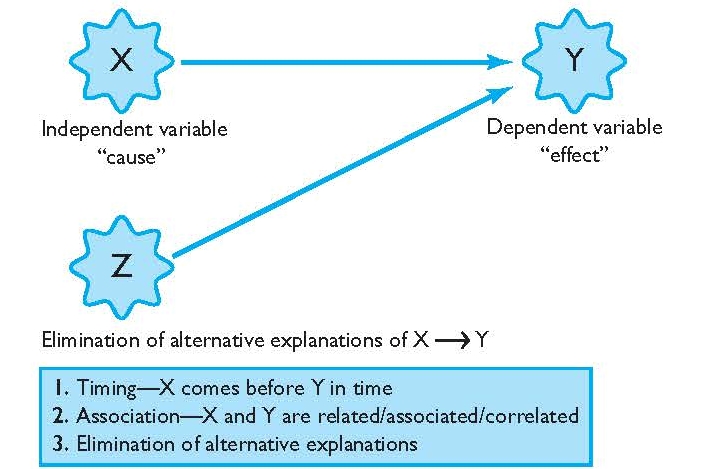
Timing The first condition for a causal relationship is timing. For a causal relationship to exist, it must be shown that the independent variable or cause (X) preceded the dependent variable or outcome (Y) in time. A decrease in domestic violence re-arrests (Y) cannot occur before participation in a domestic violence reduction program (X), if the domestic violence program is proposed to be the cause of fewer re-arrests. Ensuring that cause comes before effect is not sufficient to establish that a causal relationship exists, but it is one requirement that must be met for a causal relationship.

Association In addition to timing, there must also be an observable association between X and Y, the second necessary condition for a causal relationship. Association is also commonly referred to as covariance or correlation. When an association or correlation exits, this means there is some pattern of relationship between X and Y—as X changes by increasing or decreasing, Y also changes by increasing or decreasing. Here, the notion of X and Y increasing or decreasing can mean an actual increase/decrease in the quantity of some factor, such as an increase/decrease in the number of prison terms or days in a program or re-arrests. It can also refer to an increase/decrease in a particular category, for example, from nonparticipation in a program to participation in a program. For instance, subjects who participated in a domestic violence reduction program (X) incurred fewer domestic violence re-arrests (Y) than those who did not participate in the program. In this example, X and Y are associated—as X change s or increases from nonparticipation to participation in the domestic violence program, Y or the number of re-arrests for domestic violence decreases.

Associations between X and Y can occur in two different directions: positive or negative. A positive association means that as X increases, Y increases, or, as X decreases, Y decreases. A negative association means that as X increases, Y decreases, or, as X decreases, Y increases. In the example above, the association is negative—participation in the domestic violence program was associated with a reduction in re-arrests. This is also sometimes called an inverse relationship.

Elimination of Alternative Explanations Although participation in a domestic violence program may be associated with a reduction in re-arrests, this does not mean for certain that participation in the program was the cause of reduced re-arrests. Just as timing by itself does not imply a causal relationship, association by itself does not imply a causal relationship. For example, instead of the program being the cause of a reduction in re-arrests, perhaps several of the program participants died shortly after completion of the domestic violence program and thus were not able to engage in domestic violence (and their deaths were unknown to the researcher tracking re-arrests). Perhaps a number of the program participants moved out of state and domestic violence re-arrests occurred but were not able to be uncovered by the researcher. Perhaps those in the domestic violence program experienced some other event, such as the trauma of a natural disaster, and that experience led to a reduction in domestic violence, an event not connected to the domestic violence program. If any of these situations occurred, it might appear that the domestic violence program led to fewer re-arrests. However, the observed reduction in re-arrests can actually be attributed to a factor unrelated to the domestic violence program.

The previous discussion leads to the third and final necessary consideration in determining a causal relationship—elimination of alternative explanations. This means that the researcher must rule out any other potential explanation of the results, except for the experimental condition such as a program, policy, or practice. Accounting for or ruling out alternative explanations is much more difficult than ensuring timing and association. Ruling out all alternative explanations is difficult because there are so many potential other explanations that can wholly or partly explain the findings of a research study. This is especially true in the social sciences, where researchers are often interested in relationships explaining human behavior. Because of this difficulty, associations by themselves are sometimes mistaken as causal relationships when in fact they are spurious. A spurious relationship is one where it appears that X and Y are causally related, but the relationship is actually explained by something other than the independent variable, or X.

One only needs to go so far as the daily newspaper to find headlines and stories of mere associations being mistaken, assumed, or represented as causal relationships. For example, a newspaper headline recently proclaimed “Churchgoers live longer.”³ An uninformed consumer may interpret this headline as evidence of a causal relationship—that going to church by itself will lead to a longer life—but the astute consumer would note possible alternative explanations. For example, people who go to church may live longer because they tend to live healthier lifestyles and tend to avoid risky situations. These are two probable alternative explanations to the relationship independent of simply going to church. In another example, researchers David Kalist and Daniel Yee explored the relationship between first names and delinquent behavior in their manuscript titled “First Names and Crime: Does Unpopularity Spell Trouble?”⁴ Kalist and Lee (2009) found that unpopular names are associated with juvenile delinquency. In other words, those individuals with the most unpopular names were more likely to be delinquent than those with more popular names. According to the authors, is it not necessarily someone’s name that leads to delinquent behavior, but rather, the most unpopular names also tend to be correlated with individuals who come from disadvantaged home environments and experience a low socio-economic status of living. Rightly noted by the authors, these alternative explanations help to explain the link between someone’s name and delinquent behavior—a link that is not causal.

A frequently cited example provides more insight to the claim that an association by itself is not sufficient to prove causality. In certain cities in the United States, for example, as ice cream sales increase on a particular day or in a particular month so does the incidence of certain forms of crime. If this association were represented as a causal statement, it would be that ice cream or ice cream sales causes crime. There is an association, no doubt, and let us assume that ice cream sales rose before the increase in crime (timing). Surely, however, this relationship between ice cream sales and crime is spurious. The alternative explanation is that ice cream sales and crime are associated in certain parts of the country because of the weather. Ice cream sales tend to increase in warmer temperatures, and it just so happens that certain forms of crime tend to increase in warmer temperatures as well. This coincidence or association does not mean a causal relationship exists. Additionally, this does not mean that warm temperatures cause crime either. There are plenty of other alternative explanations for the increase in certain forms of crime and warmer temperatures.⁶ For another example of a study subject to alternative explanations, read the June 2011 news article titled “Less Crime in U.S. Thanks to Videogames.”⁷ Based on your reading, what are some other potential explanations for the crime drop other than videogames?

The preceding examples demonstrate how timing and association can be present, but the final needed condition for a causal relationship is that all alternative explanations are ruled out. While this task is difficult, the classic experimental design helps to ensure these additional explanatory factors are minimized. When other designs are used, such as quasi-experimental designs, the chance that alternative explanations emerge is greater. This potential should become clearer as we explore the organization and logic of the classic experimental design.

The Classic Experimental Design

Table 5.1 provides an illustration of the classic experimental design.¹² It is important to become familiar with the specific notation and organization of the classic experiment before a full discussion of its components and their purpose.

Major Components of the Classic Experimental Design

The classic experimental design has four major components:

1. Treatment

2. Experimental Group and Control Group

3. Pre-Test and Post-Test

4. Random Assignment

Treatment The first component of the classic experimental design is the treatment, and it is denoted by X in the classic experimental design. The treatment can be a number of things—a program, a new drug, or the implementation of a new policy. In a classic experimental design, the primary goal is to determine what effect, if any, a particular treatment had on some outcome. In this way, the treatment can also be considered the independent variable.

TABLE 5.1 | The Classic Experimental Design

Experimental Group	R	O1	X	O2
Control Group	R	O1		O2
		Pre-Test		Post-Test

Experimental Group = Group that receives the treatment

Control Group = Group that does not receive the treatment

R = Random assignment

O₁ = Observation before the treatment, or the pre-test

X = Treatment or the independent variable

O₂ = Observation after the treatment, or the post-test

Experimental and Control Groups The second component of the classic experiment is an experimental group and a control group. The experimental group receives the treatment, and the control group does not receive the treatment. There will always be at least one group that receives the treatment in experimental and quasi-experimental designs. In some cases, experiments may have multiple experimental groups receiving multiple treatments.

Pre-Test and Post-Test The third component of the classic experiment is a pre-test and a post-test. A pretest is a measure of the dependent variable or outcome before the treatment. The post-test is a measure of the dependent variable after the treatment is administered. It is important to note that the post-test is defined based on the stated goals of the program. For example, if the stated goal of a particular program is to reduce re-arrests, the post-test will be a measure of re-arrests after the program. The dependent variable also defines the pre-test. For example, if a researcher wanted to examine the impact of a domestic violence reduction program (treatment or X) on the goal of reducing re-arrests (dependent variable or Y), the pre-test would be the number of domestic violence arrests incurred before the program. Program goals may be numerous and all can constitute a post-test, and hence, the pre-test. For example, perhaps the goal of the domestic violence program is also that participants learn of different pro-social ways to handle domestic conflicts other than resorting to violence. If researchers wanted to examine this goal, the post-test might be subjects’ level of knowledge about pro-social ways to handle domestic conflicts other than violence. The pre-test would then be subjects’ level of knowledge about these pro-social alternatives to violence before they received the treatment program.

Although all designs have a post-test, it is not always the case that designs have a pre-test. This is because researchers may not have access or be able to collect information constituting the pre-test. For example, researchers may not be able to determine subjects’ level of knowledge about alternatives to domestic violence before the intervention program if the subjects are already enrolled in the domestic violence intervention program. In other cases, there may be financial barriers to collecting pre-test information. In the teen court evaluation that started this chapter, for example, researchers were not able to collect pre-test information on study participants due to the financial strain it would have placed on the agencies involved in the study.¹³ There are a number of potential reasons why a pre-test might not be available in a research study. The defining feature, however, is that the pre-test is determined by the post-test.

Random Assignment The fourth component of the classic experiment is random assignment. Random assignment refers to a process whereby members of the experimental group and control group are assigned to the two groups through a random and unbiased process. Random assignment should not be mistaken for random selection as discussed in Chapter 3. Random selection refers to selecting a smaller but representative sample from a larger population. For example, a researcher may randomly select a sample from a larger city population for the purposes of sending sample members a mail survey to determine their attitudes on crime. The goal of random selection in this example is to make sure the sample, although smaller in size than the population, accurately represents the larger population.

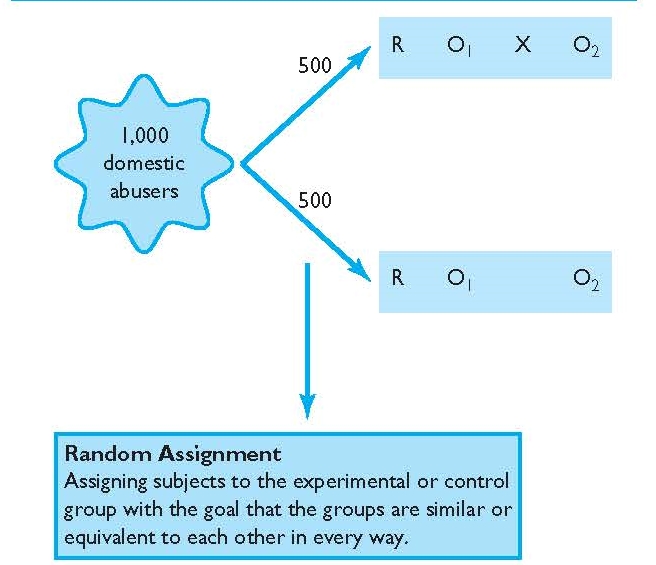
Random assignment, on the other hand, refers to the process of assigning subjects to either the experimental or control group with the goal that the groups are similar or equivalent to each other in every way (see Figure 5.2). The exception to this rule is that one group gets the treatment and the other does not (see discussion below on why equivalence is so important). Although the concept of random is similar in each, the goals are different between random selection and random assignment.¹⁴ Experimental designs all feature random assignment, but this is not true of other research designs, in particular quasi-experimental designs.

FIGURE 5.2 | Random Assignment

The classic experimental design is the foundation for all other experimental and quasi-experimental designs because it retains all of the major components discussed above. As mentioned, sometimes designs do not have a pre-test, a control group, or random assignment. Because the pre-test, control group, and random assignment are so critical to the goal of uncovering a causal relationship, if one exists, we explore them further below.

The Logic of the Classic Experimental Design

Consider a research study using the classic experimental design where the goal is to determine if a domestic violence treatment program has any effect on re-arrests for domestic violence. The randomly assigned experimental and control groups are comprised of persons who had previously been arrested for domestic violence. The pretest is a measure of the number of domestic violence arrests before the program. This is because the goal of the program is to determine whether re-arrests are impacted after the treatment. The post-test is the number of re-arrests following the treatment program.

Once randomly assigned, the experimental group members receive the domestic violence program, and the control group members do not. After the program, the researcher will compare the pre-test arrests for domestic violence of the experimental group to post-test arrests for domestic violence to determine if arrests increased, decreased, or remained constant since the start of the program. The researcher will also compare the post-test re-arrests for domestic violence between the experimental and control groups. With this example, we explore the usefulness of the classic experimental design, and the contribution of the pre-test, random assignment, and the control group to the goal of determining whether a domestic violence program reduces re-arrests.

The Pre-Test As a component of the classic experiment, the pre-test allows an examination of change in the dependent variable from before the domestic violence program to after the domestic violence program. In short, a pre-test allows the researcher to determine if re-arrests increased, decreased, or remained the same following the domestic violence program. Without a pre-test, researchers would not be able to determine the extent of change, if any, from before to after the program for either the experimental or control group.

Although the pre-test is a measure of the dependent variable before the treatment, it can also be thought of as a measure whereby the researcher can compare the experimental group to the control group before the treatment is administered. For example, the pre-test helps researchers to make sure both groups are similar or equivalent on previous arrests for domestic violence. The importance of equivalence between the experimental and control groups on previous arrests is discussed below with random assignment.

Random Assignment Random assignment helps to ensure that the experimental and control groups are equivalent before the introduction of the treatment. This is perhaps one of the most critical aspects of the classic experiment and all experimental designs. Although the experimental and control groups will be made up of different people with different characteristics, assigning them to groups via a random assignment process helps to ensure that any differences or bias between the groups is eliminated or minimized. By minimizing bias, we mean that the groups will balance each other out on all factors except the treatment. If they are balanced out on all factors prior to the administration of the treatment, any differences between the groups at the post-test must be due to the treatment—the only factor that differs between the experimental group and the control group. According to Shadish, Cook, and Campbell: “If implemented correctly, random assignment creates two or more groups of units that are probabilistically similar to each other on the average. Hence, any outcome differences that are observed between those groups at the end of a study are likely to be due to treatment, not to differences between the groups that already existed at the start of the study.”¹⁵ Considered in another way, if the experimental and control group differed significantly on any relevant factor other than the treatment, the researcher would not know if the results observed at the post-test are attributable to the treatment or to the differences between the groups.

Consider an example where 500 domestic abusers were randomly assigned to the experimental group and 500 were randomly assigned to the control group. Because they were randomly assigned, we would likely find more frequent domestic violence arrestees in both groups, older and younger arrestees in both groups, and so on. If random assignment was implemented correctly, it would be highly unlikely that all of the experimental group members were the most serious or frequent arrestees and all of the control group members were less serious and/or less frequent arrestees. While there are no guarantees, we know the chance of this happening is extremely small with random assignment because it is based on known probability theory. Thus, except for a chance occurrence, random assignment will result in equivalence between the experimental and control group in much the same way that flipping a coin multiple times will result in heads approximately 50% of the time and tails approximately 50% of the time. Over 1,000 tosses of a coin, for example, should result in roughly 500 heads and 500 tails. While there is a chance that flipping a coin 1,000 times will result in heads 1,000 times, or some other major imbalance between heads and tails, this potential is small and would only occur by chance.

The same logic from above also applies with randomly assigning people to groups, and this can even be done by flipping a coin. By assigning people to groups through a random and unbiased process, like flipping a coin, only by chance (or researcher error) will one group have more of one characteristic than another, on average. If there are no major (also called statistically significant) differences between the experimental and control group before the treatment, the most plausible explanation for the results at the post-test is the treatment.

As mentioned, it is possible by some chance occurrence that the experimental and control group members are significantly different on some characteristic prior to administration of the treatment. To confirm that the groups are in fact similar after they have been randomly assigned, the researcher can examine the pre-test if one is present. If the researcher has additional information on subjects before the treatment is administered, such as age, or any other factor that might influence post-test results at the end of the study, he or she can also compare the experimental and control group on those measures to confirm that the groups are equivalent. Thus, a researcher can confirm that the experimental and control groups are equivalent on information known to the researcher.

Being able to compare the groups on known measures is an important way to ensure the random assignment process “worked.” However, perhaps most important is that randomization also helps to ensure similarity across unknown variables between the experimental and control group. Because random assignment is based on known probability theory, there is a much higher probability that all potential differences between the groups that could impact the post-test should balance out with random assignment—known or unknown. Without random assignment, it is likely that the experimental and control group would differ on important but unknown factors and such differences could emerge as alternative explanations for the results. For example, if a researcher did not utilize random assignment and instead took the first 500 domestic abusers from an ordered list and assigned them to the experimental group and the last 500 domestic abusers and assigned them to the control group, one of the groups could be “lopsided” or imbalanced on some important characteristic that could impact the outcome of the study. With random assignment, there is a much higher likelihood that these important characteristics among the experimental and control groups will balance out because no individual has a different chance of being placed into one group versus the other. The probability of one or more characteristics being concentrated into one group and not the other is extremely small with random assignment.

To further illustrate the importance of random assignment to group equivalence, suppose the first 500 domestic violence abusers who were assigned to the experimental group from the ordered list had significantly fewer domestic violence arrests before the program than the last 500 domestic violence abusers on the list. Perhaps this is because the ordered list was organized from least to most chronic domestic abusers. In this instance, the control group would be lopsided concerning number of pre-program domestic violence arrests—they would be more chronic than the experimental group. The arrest imbalance then could potentially explain the post-test results following the domestic violence program. For example, the “less risky” offenders in the experimental group might be less likely to be re-arrested regardless of their participation in the domestic violence program, especially compared to the more chronic domestic abusers in the control group. Because of imbalances between the experimental and control group on arrests before the program was implemented, it would not be known for certain whether an observed reduction in re-arrests after the program for the experimental group was due to the program or the natural result of having less risky offenders in the experimental group. In this instance, the results might be taken to suggest that the program significantly reduces re-arrests. This conclusion might be spurious, however, for the association may simply be due to the fact that the offenders in the experimental group were much different (less frequent offenders) than the control group. Here, the program may have had no effect—the experimental group members may have performed the same regardless of the treatment because they were low-level offenders.

The example above suggests that differences between the experimental and control groups based on previous arrest records could have a major impact on the results of a study. Such differences can arise with the lack of random assignment. If subjects were randomly assigned to the experimental and control group, however, there would be a much higher probability that less frequent and more frequent domestic violence arrestees would have been found in both the experimental and control groups and the differences would have balanced out between the groups—leaving any differences between the groups at the post-test attributable to the treatment only.

In summary, random assignment helps to ensure that the experimental and control group members are balanced or equivalent on all factors that could impact the dependent variable or post-test—known or unknown. The only factor they are not balanced or equal on is the treatment. As such, random assignment helps to isolate the impact of the treatment, if any, on the post-test because it increases confidence that the only difference between the groups should be that one group gets the treatment and the other does not. If that is the only difference between the groups, any change in the dependent variable between the experimental and control group must be attributed to the treatment and not an alternative explanation, such as significant arrest history imbalance between the groups (refer to Figure 5.2). This logic also suggests that if the experimental group and control group are imbalanced on any factor that may be relevant to the outcome, that factor then becomes a potential alternative explanation for the results—an explanation that reduces the researcher’s ability to isolate the real impact of the treatment.

The Control Group The presence of an equivalent control group (created through random assignment) also gives the researcher more confidence that the findings at the post-test are due to the treatment and not some other alternative explanation. This logic is perhaps best demonstrated by considering how interpretation of results is affected without a control group. Absent an equivalent control group, it cannot be known whether the results of the study are due to the program or some other factor. This is because the control group provides a baseline of comparison or a “control.” For example, without a control group, the researcher may find that domestic violence arrests declined from pre-test to post-test. But the researcher would not be able to definitely attribute that finding to the program without a control group. Perhaps the single experimental group incurred fewer arrests because they matured over their time in the program, regardless of participation in the domestic violence program. Having a randomly assigned control group would allow this consideration to be eliminated, because the equivalent control group would also have naturally matured if that was the case.

Because the control group is meant to be similar to the experimental group on all factors with the exception that the experimental group receives the treatment, the logic is that any differences between the experimental and control group after the treatment must then be attributable only to the treatment itself—everything else occurs equally in both the experimental and control groups and thus cannot be the cause of results. The bottom line is that a control group allows the researcher more confidence to attribute any change in the dependent variable from pre- to post-test and between the experimental and control groups to the treatment—and not another alternative explanation. Absent a control group, the researcher would have much less confidence in the results.

Knowledge about the major components of the classic experimental design and how they contribute to an understanding of cause and effect serves as an important foundation for studying different types of experimental and quasi-experimental designs and their organization. A useful way to become familiar with the components of the experimental design and their important role is to consider the impact on the interpretation of results when one or more components are lacking. For example, what if a design lacked a pre-test? How could this impact the interpretation of post-test results and knowledge about the comparability of the experimental and control group? What if a design lacked random assignment? What are some potential problems that could occur and how could those potential problems impact interpretation of results? What if a design lacked a control group? How does the absence of an equivalent control group affect a researcher’s ability to determine the unique effects of the treatment on the outcomes being measured? The ability to discuss the contribution of a pre-test, random assignment, and a control group—and what is the impact when one or more of those components is absent from a research design—is the key to understanding both experimental and quasi-experimental designs that will be discussed in the remainder of this chapter. As designs lose these important parts and transform from a classic experiment to another experimental design or to a quasi-experiment, they become less useful in isolating the impact that a treatment has on the dependent variable and allow more room for alternative explanations of the results.

One more important point must be made before further delving into experimental and quasi-experimental designs. This point is that rarely, if ever, will the average consumer of research be exposed to the symbols or specific language of the classic experiment, or other experimental and quasi-experimental designs examined in this chapter. In fact, it is unlikely that the average consumer will ever be exposed to the terms pre-test, post-test, experimental group, or random assignment in the popular media, among other terms related to experimental and quasi-experimental designs. Yet, consumers are exposed to research results produced from these and other research designs every day. For example, if a national news organization or your regional newspaper reported a story about the effectiveness of a new drug to reduce cholesterol or the effects of different diets on weight loss, it is doubtful that the results would be reported as produced through a classic experimental design that used a control group and random assignment. Rather, these media outlets would use generally nonscientific terminology such as “results of an experiment showed” or “results of a scientific experiment indicated” or “results showed that subjects who received the new drug had greater cholesterol reductions than those who did not receive the new drug.” Even students who regularly search and read academic articles for use in course papers and other projects will rarely come across such design notation in the research studies they utilize. Depiction of the classic experimental design, including a discussion of its components and their function, simply illustrates the organization and notation of the classic experimental design. Unfortunately, the average consumer has to read between the lines to determine what type of design was used to produce the reported results. Understanding the key components of the classic experimental design allows educated consumers of research to read between those lines.

Variations on the Experimental Design

The classic experimental design is the foundation upon which all experimental and quasi-experimental designs are based. As such, it can be modified in numerous ways to fit the goals (or constraints) of a particular research study. Below are two variations of the experimental design. Again, knowledge about the major components of the classic experiment, how they contribute to an explanation of results, and what the impact is when one or more components are missing provides an understanding of all other experimental designs.

Post-Test Only Experimental Design

The post-test only experimental design could be used to examine the impact of a treatment program on school disciplinary infractions as measured or operationalized by referrals to the principal’s office (see Table 5.2). In this design, the researcher randomly assigns a group of discipline problem students to the experimental group and control group by flipping a coin—heads to the experimental group and tails to the control group. The experimental group then enters the 3-month treatment program. After the program, the researcher compares the number of referrals to the principal’s office between the experimental and control groups over some period of time, for example, discipline referrals at 6 months after the program. The researcher finds that the experimental group has a much lower number of referrals to the principal’s office in the 6 month follow-up period than the control group.

TABLE 5.2 | Post-Test Only Experimental Design

Experimental Group	R	X	O
Control Group	R		O
			Post-Test

Several issues arise in this example study. The researcher would not know if discipline problems decreased, increased, or stayed the same from before to after the treatment program because the researcher did not have a count of disciplinary referrals prior to the treatment program (e.g., a pre-test). Although the groups were randomly assigned and are presumed equivalent, the absence of a pre-test means the researcher cannot confirm that the experimental and control groups were equivalent before the treatment was administered, particularly on the number of referrals to the principal’s office. The groups could have differed by a chance occurrence even with random assignment, and any such differences between the groups could potentially explain the post-test difference in the number of referrals to the principal’s office. For example, if the control group included much more serious or frequent discipline problem students than the experimental group by chance, this difference might explain the lower number of referrals for the experimental group, not that the treatment produced this result.

Experimental Design with Two Treatments and a Control Group

This design could be used to determine the impact of boot camp versus juvenile detention on post-release recidivism (see Table 5.3). Recidivism in this study is operationalized as re-arrest for delinquent behavior. First, a population of known juvenile delinquents is randomly assigned to either boot camp, juvenile detention, or a control condition where they receive no sanction. To accomplish random assignment to groups, the researcher places the names of all youth into a hat and assigns the groups in order. For example, the first name pulled goes into experimental group 1, the next into experimental group 2, and the next into the control group, and so on. Once randomly assigned, the experimental group youth receive either boot camp or juvenile detention for a period of 3 months, whereas members of the control group are released on their own recognizance to their parents. At the end of the experiment, the researcher compares the re-arrest activity of boot camp participants to detention delinquents to control group members during a 6-month follow-up period.

TABLE 5.3 | Experimental Design with Two Treatments and a Control Group

Experimental Group	R	O1	X1	O2
Experimental Group	R	O1	X2	O2
Control Group	R	O1		O2
		Pre-Test		Post-Test

This design has several advantages. First, it includes all major components of the classic experimental design, and simply adds an additional treatment for comparison purposes. Random assignment was utilized and this means that the groups have a higher probability of being equivalent on all factors that could impact the post-test. Thus, random assignment in this example helps to ensure the only differences between the groups are the treatment conditions. Without random assignment, there is a greater chance that one group of youth was somehow different, and this difference could impact the post-test. For example, if the boot camp youth were much less serious and frequent delinquents than the juvenile detention youth or control group youth, the results might erroneously show that the boot camp reduced recidivism when in fact the youth in boot camp may have been the “best risks”—unlikely to get re-arrested with or without boot camp. The pre-test in the example above allows the researcher to determine change in re-arrests from pretest to post-test. Thus, the researcher can determine if delinquent behavior, as measured by re-arrest, increased, decreased, or remained constant from pre- to post-test. The pre-test also allows the researcher to confirm that the random assignment process resulted in equivalent groups based on the pre-test. Finally, the presence of a control group allows the researcher to have more confidence that any differences in the post-test are due to the treatment. For example, if the control group had more re-arrests than the boot camp or juvenile detention experimental groups 6 months after their release from those programs, the researcher would have more confidence that the programs produced fewer re-arrests because the control group members were the same as the experimental groups; the only difference was that they did not receive a treatment.

The one key feature of experimental designs is that they all retain random assignment. This is why they are considered “experimental” designs. Sometimes, however, experimental designs lack a pre-test. Knowledge of the usefulness of a pre-test demonstrates the potential problems with those designs where it is missing. For example, in the post-test only experimental design, a researcher would not be able to make a determination of change in the dependent variable from pre- to post-test. Perhaps most importantly, the researcher would not be able to confirm that the experimental and control groups were in fact equivalent on a pre-test measure before the introduction of the treatment. Even though both groups were randomly assigned, and probability theory suggests they should be equivalent, without a pre-test measure the researcher could not confirm similarity because differences could occur by chance even with random assignment. If there were any differences at the post-test between the experimental group and control group, the results might be due to some explanation other than the treatment, namely that the groups differed prior to the administration of the treatment. The same limitation could apply in any form of experimental design that does not utilize a pre-test for conformational purposes.

Understanding the contribution of a pre-test to an experimental design shows that it is a critical component. It provides a measure of change and also gives the researcher more confidence that the observed results are due to the treatment, and not some difference between the experimental and control groups. Despite the usefulness of a pre-test, however, perhaps the most critical ingredient of any experimental design is random assignment. It is important to note that all experimental designs retain random assignment.

Experimental Designs Are Rare in Criminal Justice and Criminology

The classic experiment is the foundation for other types of experimental and quasi-experimental designs. The unfortunate reality, however, is that the classic experiment, or other experimental designs, are few and far between in criminal justice.²⁰ Recall that one of the major components of an experimental design is random assignment. Achieving random assignment is often a barrier to experimental research in criminal justice. Achieving random assignment might, for example, require the approval of the chief (or city council or both) of a major metropolitan police agency to allow researchers to randomly assign patrol officers to certain areas of a city and/or randomly assign police officer actions. Recall the MDVE. This experiment required the full cooperation of the chief of police and other decision-makers to allow researchers to randomly assign police actions. In another example, achieving random assignment might require a judge to randomly assign a group of youthful offenders to a certain juvenile court sanction (experimental group), and another group of similar youthful offenders to no sanction or an alternative sanction as a control group.²¹ In sum, random assignment typically requires the cooperation of a number of individuals and sometimes that cooperation is difficult to obtain.

Even when random assignment can be accomplished, sometimes it is not implemented correctly and the random assignment procedure breaks down. This is another barrier to conducting experimental research. For example, in the MDVE, researchers randomly assigned officer responses, but the officers did not always follow the assigned course of action. Moreover, some believe that the random assignment of criminal justice programs, sentences, or randomly assigning officer responses may be unethical in certain circumstances, and even a violation of the rights of citizens. For example, some believe it is unfair when random assignment results in some delinquents being sentenced to boot camp while others get assigned to a control group without any sanction at all or a less restrictive sanction than boot camp. In the MDVE, some believe it is unfair that some suspects were arrested and received an official record whereas others were not arrested for the same type of behavior. In other cases, subjects in the experimental group may receive some benefit from the treatment that is essentially denied to the control group for a period of time and this can become an issue as well.

There are other important reasons why random assignment is difficult to accomplish. Random assignment may, for example, involve a disruption of the normal procedures of agencies and their officers. In the MDVE, officers had to adjust their normal and established routine, and this was a barrier at times in that study. Shadish, Cook, and Campbell also note that random assignment may not always be feasible or desirable when quick answers are needed.²² This is because experimental designs sometimes take a long time to produce results. In addition to the time required in planning and organizing the experiment, and treatment delivery, researchers may need several months if not years to collect and analyze the data before they have answers. This is particularly important because time is often of the essence in criminal justice research, especially in research efforts testing the effect of some policy or program where it is not feasible to wait years for answers. Waiting for the results of an experimental design means that many policy-makers may make decisions without the results.

Quasi-Experimental Designs

In general terms, quasi-experiments include a group of designs that lack random assignment. Quasi-experiments may also lack other parts, such as a pre-test or a control group, just like some experimental designs. The absence of random assignment, however, is the ingredient that transforms an otherwise experimental design into a quasi-experiment. Lacking random assignment is a major disadvantage because it increases the chances that the experimental and control groups differ on relevant factors before the treatment—both known and unknown—differences that may then emerge as alternative explanations of the outcomes.

Just like experimental designs, quasi-experimental designs can be organized in many different ways. This section will discuss three types of quasi-experiments: nonequivalent group design, one-group longitudinal design, and two-group longitudinal design.

Nonequivalent Group Design

The nonequivalent group design is perhaps the most common type of quasi-experiment.²³ Notice that it is very similar to the classic experimental design with the exception that it lacks random assignment (see Table 5.4). Additionally, what was labeled the experimental group in an experimental design is sometimes called the treatment group in the nonequivalent group design. What was labeled the control group in the experimental design is sometimes called the comparison group in the nonequivalent group design. This terminological distinction is an indicator that the groups were not created through random assignment.

TABLE 5.4 | Nonequivalent Group Design

Treatment Group	NR	O1	X	O2
Comparison Group	NR	O1		O2
		Pre-Test		Post-Test

NR = Not Randomly assigned

One of the main problems with the nonequivalent group design is that it lacks random assignment, and without random assignment, there is a greater chance that the treatment and comparison groups may be different in some way that can impact study results. Take, for example, a nonequivalent group design where a researcher is interested in whether an aggression-reduction treatment program can reduce inmate-on-inmate assaults in a prison setting. Assume that the researcher asked for inmates who had previously been involved in assaultive activity to volunteer for the aggression-reduction program. Suppose the researcher placed the first 50 volunteers into the treatment group and the next 50 volunteers into the comparison group. Note that this method of assignment is not random but rather first come, first serve.

Because the study utilized volunteers and there was no random assignment, it is possible that the first 50 volunteers placed into the treatment group differed significantly from the last 50 volunteers who were placed in the comparison group. This can lead to alternative explanations for the results. For example, if the treatment group was much younger than the comparison group, the researcher may find at the end of the program that the treatment group still maintained a higher rate of infractions than the comparison group—even after the aggression-reduction program! The conclusion might be that the aggression program actually increased the level of violence among the treatment group. This conclusion would likely be spurious and may be due to the age differential between the treatment and comparison groups. Indeed, research has revealed that younger inmates are significantly more likely to engage in prison assaults than older inmates. The fact that the treatment group incurred more assaults than the comparison group after the aggression-reduction program may only relate to the age differential between the groups, not that the program had no effect or that it somehow may have increased aggression. The previous example highlights the importance of random assignment and the potential problems that can occur in its absence.

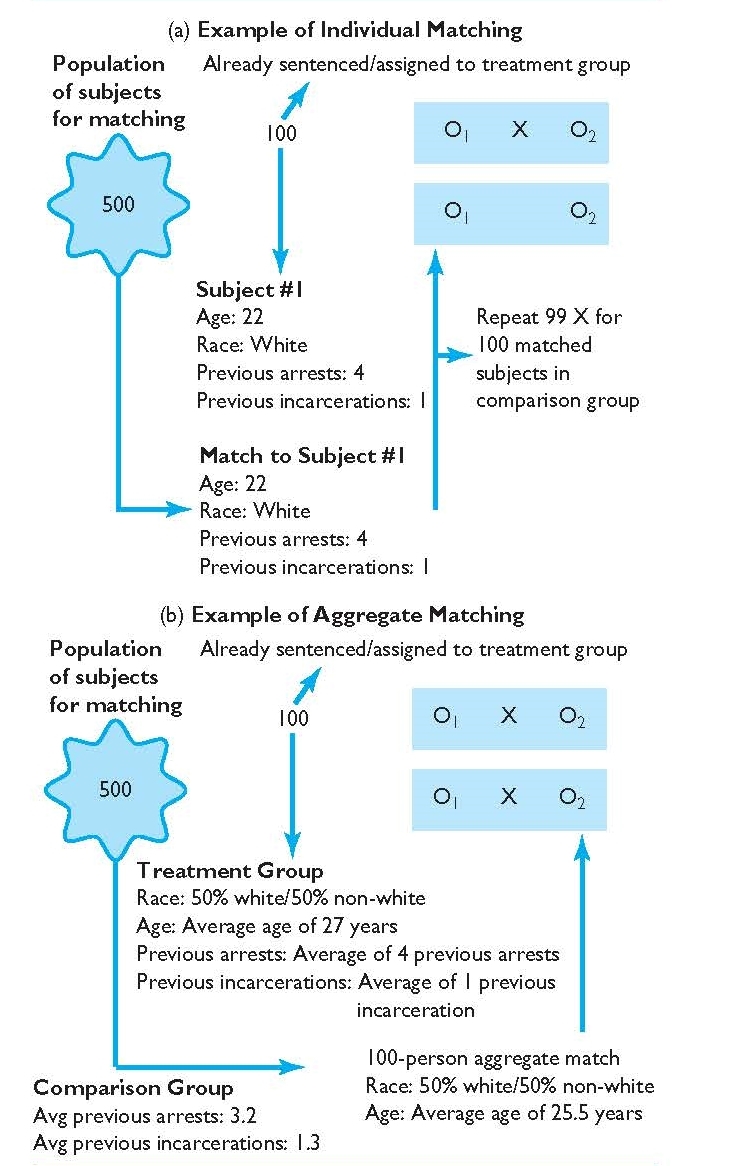
Although researchers who utilize a quasi-experimental design are not able to randomly assign their subjects to groups, they can employ other techniques in an attempt to make the groups as equivalent as possible on known or measured factors before the treatment is given. In the example above, it is likely that the researcher would have known the age of inmates, their prior assault record, and various other pieces of information (e.g., previous prison stays). Through a technique called matching, the researcher could make sure the treatment and comparison groups were “matched” on these important factors before administering the aggression reduction program to the treatment group. This type of matching can be done individual to individual (e.g., subject #1 in treatment group is matched to a selected subject #1 in comparison group on age, previous arrests, gender), or aggregately, such that the comparison group is similar to the treatment group overall (e.g., average ages between groups are similar, equal proportions of males and females). Knowledge of these and other important variables, for example, would allow the researcher to make sure that the treatment group did not have heavy concentrations of younger or more frequent or serious offenders than the comparison group—factors that are related to assaultive activity independent of the treatment program. In short, matching allows the researcher some control over who goes into the treatment and comparison groups so as to balance these groups on important factors absent random assignment. If unbalanced on one or more factors, these factors could emerge as alternative explanations of the results. Figure 5.3 demonstrates the logic of matching both at the individual and aggregate level in a quasi-experimental design.

Matching is an important part of the nonequivalent group design. By matching, the researcher can approximate equivalence between the groups on important variables that may influence the post-test. However, it is important to note that a researcher can only match subjects on factors that they have information about—a researcher cannot match the treatment and comparison group members on factors that are unmeasured or otherwise unknown but which may still impact outcomes. For example, if the researcher has no knowledge about the number of previous incarcerations, the researcher cannot match the treatment and comparison groups on this factor. Matching also requires that the information used for matching is valid and reliable, which is not always the case. Agency records, for example, are notorious for inconsistencies, errors, omissions, and for being dated, but are often utilized for matching purposes. Asking survey questions to generate information for matching (for example, how many times have you been incarcerated?) can also be problematic because some respondents may lie, forget, or exaggerate their behavior or experiences.

In addition to the above considerations, the more factors a researcher wishes to match the group members on, the more difficult it becomes to find appropriate matches. Matching on prior arrests or age is less complex than matching on several additional pieces of information. Finally, matching is never considered superior to random assignment when the goal is to construct equitable groups. This is because there is a much higher likelihood of equivalence with random assignment on factors that are both measured and unknown to the researcher. Thus, the results produced from a nonequivalent group design, even with matching, are at a greater risk of alternative explanations than an experimental design that features random assignment.

FIGURE 5.3 | (a) Individual Matching (b) Aggregate Matching

The previous discussion is not to suggest that the nonequivalent group design cannot be useful in answering important research questions. Rather, it is to suggest that the nonequivalent group design, and hence any quasi-experiment, is more susceptible to alternative explanations than the classic experimental design because of the absence of random assignment. As a result, a researcher must be prepared to rule out potential alternative explanations. Quasi-experimental designs that lack a pre-test or a comparison group are even less desirable than the nonequivalent group design and are subject to additional alternative explanations because of these missing parts. Although the quasi-experiment may be all that is available and still can serve as an important design in evaluating the impact of a particular treatment, it is not preferable to the classic experiment. Researchers (and consumers) must be attuned to the potential issues of this design so as to make informed conclusions about the results produced from such research studies.

One-Group Longitudinal Design

Like all experimental designs, the quasi-experimental design can come in a variety of forms. The second quasi-experimental design (above) is the one-group longitudinal design (also called a simple interrupted time series design).²⁶ An examination of this design shows that it lacks both random assignment and a comparison group (see Table 5.5). A major difference between this design and others we have covered is that it includes multiple pre-test and post-test observations.

TABLE 5.5 | One-Group Longitudinal Design

Treatment	NR	O1	O1	O1	O1	X	O2	O2	O2	O2
			Pre-Test					Post-Test

The one-group longitudinal design is useful when researchers are interested in exploring longer-term patterns. Indeed, the term longitudinal generally means “over time”—repeated measurements of the pre-test and post-test over time. This is different from cross-sectional designs, which examine the pre-test and post-test at only one point in time (e.g., at a single point before the application of the treatment and at a single point after the treatment). For example, in the nonequivalent group design and the classic experimental design previously examined, both are cross-sectional because pre-tests and post-tests are measured at one point in time (e.g., at a point 6 months after the treatment). Yet, these designs could easily be considered longitudinal if researchers took repeated measures of the pre-test and post-test.

The organization of the one-group longitudinal design is to examine a baseline of several pre-test observations, introduce a treatment or intervention, and then examine the post-test at several different time intervals. As organized, this design is useful for gauging the impact that a particular program, policy, or law has, if any, and how long the treatment impact lasts. Consider an example whereby a researcher is interested in gauging the impact of a tobacco ban on inmate-on-inmate assaults in a prison setting. This is an important question, for recent years have witnessed correctional systems banning all tobacco products from prison facilities. Correctional administrators predicted that there would be a major increase of inmate-on-inmate violence once the bans took effect. The one-group longitudinal design would be one appropriate design to examine the impact of banning tobacco on inmate assaults.

To construct this study using the one-group longitudinal design, the researcher would first examine the rate of inmate-on-inmate assaults in the prison system (or at an individual prison, a particular cellblock, or whatever the unit of analysis) prior to the removal of tobacco. This is the pre-test, or a baseline of assault activity before the ban goes into effect. In the design presented above, perhaps the researcher would measure the level of assaults in the preceding four months prior to the tobacco ban. When establishing a pre-test baseline, the general rule is that, in a longitudinal design, the more time utilized, both in overall time and number of intervals, the better. For example, the rate of assaults in the preceding month is not as useful as an entire year of data on inmate assaults prior to the tobacco ban. Next, once the tobacco ban is implemented, the researcher would then measure the rate of inmate assaults in the coming months to determine what impact the ban had on inmate-on-inmate assaults. This is shown in Table 5.5 as the multiple post-test measures of assaults. Assaults may increase, decrease, or remain constant from the pre-test baseline over the term of the post-test.

If assaults increased at the same time as the ban went into effect, the researcher might conclude that the increase was due only to the tobacco ban. But, could there be alternative explanations? The answer to this question is yes, there may be other plausible explanations for the increase even with several months of pre-test data. Unfortunately, without a comparison group there is no way for the researcher to be certain if the increase in assaults was due to the tobacco ban, or some other factor that may have spurred the increase in assaults and happened at the same time as the tobacco ban. What if assaults decreased after the tobacco ban went into effect? In this scenario, because there is no comparison group, the researcher would still not know if the results would have happened anyway without the tobacco ban. In these instances, the lack of a comparison group prevents the researcher from confidently attributing the results to the tobacco ban, and interpretation is subject to numerous alternative explanations.

Two-Group Longitudinal Design

A remedy for the previous situation would be to introduce a comparison group (see Table 5.6). Prior to the full tobacco ban, suppose prison administrators conducted a pilot program at one prison to provide insight as to what would happen once the tobacco ban went into effect systemwide. To conduct this pilot, the researcher identified one prison. At this prison, the researcher identified two different cellblocks, C-Block and D-Block. C-Block constitutes the treatment group, or the cellblock of inmates who will have their tobacco taken away. D-Block is the comparison group—inmates in this cellblock will retain their tobacco privileges during the course of the study and during a determined follow-up period to measure post-test assaults (e.g., 12-months). This is a two-group longitudinal design (also sometimes called a multiple interrupted time series design), and adding a comparison group makes this design superior to the one-group longitudinal design.

TABLE 5.6 | Two-Group Longitudinal Design

Treatment	NR	O1	O1	O1	O1	X	O2	O2	O2	O2
Comparison	NR	O1	O1	O1	O1		O2	O2	O2	O2
			Pre-Test					Post-Test

The usefulness of adding a comparison group to the study means that the researcher can have more confidence that the results at the post-test are due to the tobacco ban and not some alternative explanation. This is because any difference in assaults at the post-test between the treatment and comparison group should be attributed to the only difference between them, the tobacco ban. For this interpretation to hold, however, the researcher must be sure that C-Block and D-Block are similar or equivalent on all factors that might influence the post-test. There are many potential factors that should be considered. For example, the researcher will want to make sure that the same types of inmates are housed in both cellblocks. If a chronic group of assaultive inmates constitutes members of C-Block, but not D-Block, this differential could explain the results, not the treatment.

The researcher might also want to make sure equitable numbers of tobacco and non-tobacco users are found in each cellblock. If very few inmates in C-Block are smokers, the real effect of removing tobacco may be hidden. The researcher might also examine other areas where potential differences might arise, for example, that both cellblocks are staffed with equal numbers of officers, that officers in each cellblock tend to resolve inmate disputes similarly, and other potential issues that could influence post-test measure of assaults. Equivalence could also be ensured by comparing the groups on additional evidence before the ban takes effect: number of prior prison sentences, time served in prison, age, seriousness of conviction crime, and other factors that might relate to assaultive behavior, regardless of the tobacco ban. Moreover, the researcher should ensure that inmates in C-Block do not know that their D-Block counterparts are still allowed tobacco during the pilot study, and vice versa. If either group knows about the pilot program being an experiment, they might act differently than normal, and this could become an explanation of results. Additionally, the researchers might also try to make sure that C-Block inmates are completely tobacco free after the ban goes into effect—that they do not hoard, smuggle, or receive tobacco from officers or other inmates during the tobacco ban in or outside of the cellblock. If these and other important differences are accounted for at the individual and cellblock level, the researcher will have more confidence that any differences in assaults at the post-test between the treatment and comparison groups are related to the tobacco ban, and not some other difference between the two groups or the two cellblocks.

The addition of a comparison group aids in the ability of the researcher to isolate the true impact of a tobacco ban on inmate-on-inmate assaults. All factors that influence the treatment group should also influence the comparison group because the groups are made up of equivalent individuals in equivalent circumstances, with the exception of the tobacco ban. If this is the only difference, the results can be attributed to the ban. Although the addition of the comparison group in the two-group longitudinal design provides more confidence that the findings are attributed to the tobacco ban, the fact that this design lacks randomization means that alternative explanations cannot be completely ruled out—but they can be minimized. This example also suggests that the quasi-experiment in this instance may actually be preferable to an experimental design—noting the realities of prison administration. For example, prison inmates are not typically randomly assigned to different cellblocks by prison officers. Moreover, it is highly unlikely that a prison would have two open cellblocks waiting for a researcher to randomly assign incoming inmates to the prison for a tobacco ban study. Therefore, it is likely there would be differences among the groups in the quasi-experiment.

Fortunately, if differences between the groups are present, the researcher can attempt to determine their potential impact before interpretation of results. The researcher can also use statistical models after the ban takes effect to determine the impact of any differences between the groups on the post-test. While the two-group longitudinal quasi-experiment just discussed could also take the form of an experimental design, if random assignment could somehow be accomplished, the previous discussion provides one situation where an experimental design might be appropriate and desired for a particular research question, but would not be realistic considering the many barriers.

The Threat of Alternative Explanations

Alternative explanations are those factors that could explain the post-test results, other than the treatment. Throughout this chapter, we have noted the potential for alternative explanations and have given several examples of explanations other than the treatment. It is important to know that potential alternative explanations can arise in any research design discussed in this chapter. However, alternative explanations often arise because some design part is missing, for example, random assignment, a pre-test, or a control or comparison group. This is especially true in criminal justice where researchers often conduct field studies and have less control over their study conditions than do researchers who conduct experiments under highly controlled laboratory conditions. A prime example of this is the tobacco ban study, where it would be difficult for researchers to ensure that C-Block inmates, the treatment group, were completely tobacco free during the course of the study.

Alternative explanations are typically referred to as threats to internal validity. In this context, if an experiment is internally valid, it means that alternative explanations have been ruled out and the treatment is the only factor that produced the results. If a study is not internally valid, this means that alternative explanations for the results exist or potentially exist. In this section, we focus on some common alternative explanations that may arise in experimental and quasi-experimental designs.²⁷

Selection Bias

One of the more common alternative explanations that may occur is selection bias. Selection bias generally indicates that the treatment group (or experimental group) is somehow different from the comparison group (or control group) on a factor that could influence the post-test results. Selection bias is more often a threat in quasi-experimental designs than experimental designs due to the lack of random assignment. Suppose in our study of the prison tobacco ban, members of C-Block were substantially younger than members of D-Block, the comparison group. Such an imbalance between the groups would mean the researcher would not know if the differences in assaults are real (meaning the result of the tobacco ban) or a result of the age differential. Recall that research shows that younger inmates are more assaultive than older inmates and so we would expect more assaults among the younger offenders independent of the tobacco ban.

In a quasi-experiment, selection bias is perhaps the most prevalent type of alternative explanation and can seriously compromise results. Indeed, many of the examples above have referred to potential situations where the groups are imbalanced or not equivalent on some important factor. Although selection bias is a common threat in quasi-experimental designs because of lack of random assignment, and can be a threat in experimental designs because the groups could differ by chance alone or the practice of randomization was not maintained throughout the study (see Classics in CJ Research-MDVE above), a researcher may be able to detect such differentials. For example, the researcher could detect such differences by comparing the groups on the pre-test or other types of information before the start of the study. If differences were found, the researcher could take measures to correct them. The researcher could also use a statistical model that could account or control for differences between the groups and isolate the impact of the treatment, if any. This discussion is beyond the scope of this text but would be a potential way to deal with selection bias and estimate the impact of this bias on study results. The researcher could also, if possible, attempt to re-match the groups in a quasi-experiment or randomly assign the groups a second time in an experimental design to ensure equivalence. At the least, the researcher could recognize the group differences and discuss their potential impact on the results. Without a pre-test or other pre-study information on study participants, however, such differences might not be able to be detected and, therefore, it would be more difficult to determine how the differences, as a result of selection bias, influenced the results.

History

Another potential alternative explanation is history. History refers to any event experienced differently by the treatment and comparison groups in the time between the pre-test and the post-test that could impact results. Suppose during the course of the tobacco ban study several riots occurred on D-Block, the comparison group. Because of the riots, prison officers “locked down” this cellblock numerous times. Because D-Block inmates were locked down at various times, this could have affected their ability to otherwise engage in inmate assaults. At the end of the study, the assaults in D-Block might have decreased from their pre-test levels because of the lockdowns, whereas in C-Block assaults may have occurred at their normal pace because there was not a lockdown, or perhaps even increased from the pretest because tobacco was also taken away. Even if the tobacco ban had no effect and assaults remained constant in C-Block from pre- to post-test, the lockdown in D-Block might make it appear that the tobacco ban led to increased assaults in C-Block. Thus, the researcher would not know if the post-test results for the C-Block treatment group were attributable to the tobacco ban or the simple fact that D-Block inmates were locked down and their assault activity was artificially reduced. In this instance, the comparison group becomes much less useful because the lockdown created a historical factor that imbalanced the groups during the treatment phase and nullified the comparison.

Maturation

Another potential alternative explanation is maturation. Maturation refers to the natural biological, psychological, or emotional processes we all experience as time passes—aging, becoming more or less intelligent, becoming bored, and so on. For example, if a researcher was interested in the effect of a boot camp on recidivism for juvenile offenders, it is possible that over the course of the boot camp program the delinquents naturally matured as they aged and this produced the reduction in recidivism—not that the boot camp somehow led to this reduction. This threat is particularly applicable in situations that deal with populations that rapidly change over a relatively short period of time or when a treatment lasts a considerable period of time. However, this threat could be eliminated with a comparison group that is similar to the treatment group. This is because the maturation effects would occur in both groups and the effect of the boot camp, if any, could be isolated. This assumes, however, that the groups are matched and equitable on factors subject to the maturation process, such as age. If not, such differentials could be an alternative explanation of results. For example, if the treatment and comparison groups differ by age, on average, this could mean that one group changes or matures at a different rate than the other group. This differential rate of change or maturation as a result of the age differential could explain the results, not the treatment. This example demonstrates how selection bias and maturation can interact at the same time as alternative explanations. This example also suggests the importance of an equivalent control or comparison group to eliminate or minimize the impact of maturation as an alternative explanation.

Attrition or Subject Mortality

Attrition or subject mortality is another typical alternative explanation. Attrition refers to differential loss in the number or type of subjects between the treatment and comparison groups and can occur in both experimental and quasi-experimental designs. Suppose we wanted to conduct a study to determine who is the better research methods professor among the authors of this textbook. Let’s assume that we have an experimental design where students were randomly assigned to professor 1, professor 2, or professor 3. By randomly assigning students to each respective professor, there is greater probability that the groups are equivalent and thus there are no differences between the three groups with one exception—the professor they receive and his or her particular teaching and delivery style. This is the treatment. Let’s also assume that the professors will be administering the same tests and using the same textbook. After the group members are randomly assigned, a pre-treatment evaluation shows the groups are in fact equivalent on all important known factors that could influence post-test scores, such as grade point average, age, time in school, and exposure to research methods concepts. Additionally, all groups scored comparably on a pre-test of knowledge about research methods, thus there is more confidence that the groups are in fact equivalent.

At the conclusion of the study, we find that professor 2’s group has the lowest final test scores of the three. However, because professor 2 is such an outstanding professor, the results appear odd. At first glance, the researcher thinks the results could have been influenced by students dropping out of the class. For example, perhaps several of professor 2’s students dropped the course but none did from the classes of professor 1 or 3. It is revealed, however, that an equal number of students dropped out of all three courses before the post-test and, therefore, this could not be the reason for the low scores in professor 2’s course. Upon further investigation, however, the researcher finds that although an equal number of students dropped out of each class, the dropouts in professor 2’s class were some of his best students. In contrast, those who dropped out of professor 1’s and professor 3’s courses were some of their poorest students. In this example, professor 2 appears to be the least effective teacher. However, this result appears to be due to the fact that his best students dropped out, and this highly influenced the final test average for his group. Although there was not a differential loss of subjects in terms of numbers (which can also be an attrition issue), there was differential loss in the types of students. This differential loss, not the teaching style, is an alternative explanation of the results.

Testing or Testing Bias

Another potential alternative explanation is testing or testing bias. Suppose that after the pre-test of research methods knowledge, professor 1 and professor 3 reviewed the test with their students and gave them the correct answers. Professor 2 did not. The fact that professor l’s and professor 3’s groups did better on the post-test final exam may be explained by the finding that students in those groups remembered the answers to the pre-test, were thus biased at the pre-test, and this artificially inflated their post-test scores. Testing bias can explain the results because students in groups 1 and 3 may have simply remembered the answers from the pre-test review. In fact, the students in professor l’s and 3’s courses may have scored high on the post-test without ever having been exposed to the treatment because they were biased at the pre-test.

Instrumentation

Another alternative explanation that can arise is instrumentation. Instrumentation refers to changes in the measuring instrument from pre- to post-test. Using the previous example, suppose professors 1 and 3 did not give the same final exam as professor 2. For example, professors 1 and 3 changed the final exam and professor 2 kept the final exam the same as the pretest. Because professors 1 and 3 changed the exam, and perhaps made it easier or somehow different from the pre-test exam, results that showed lower scores for professor 2’s students may be related only to instrumentation changes from pre- to post-test. Obviously, to limit the influence of instrumentation, researchers should make sure that instruments remain consistent from pre- to post-test.

Reactivity

A final alternative explanation is reactivity. Reactivity occurs when members of the treatment or experimental group change their behavior simply as a result of being part of a study. This is akin to the finding that people tend to change their behavior when they are being watched or are aware they are being studied. If members of the experiment know they are part of an experiment and are being studied and watched, it is possible that their behavior will change independent of the treatment. If this occurs, the researcher will not know if the behavior change is the result of the treatment, or simply a result of being part of a study. For example, suppose a researcher wants to determine if a boot camp program impacts the recidivism of delinquent offenders. Members of the experimental group are sentenced to boot camp and members of the control group are released on their own recognizance to their parents. Because members of the experimental group know they are part of the experiment, and hence being watched closely after they exit boot camp, they may artificially change their behavior and avoid trouble. Their change of behavior may be totally unrelated to boot camp, but rather, to their knowledge of being part of an experiment.

Other Potential Alternative Explanations

The above discussion provided some typical alternative explanations that may arise with the designs discussed in this chapter. There are, however, other potential alternative explanations that may arise. These alternative explanations arise only when a control or comparison group is present.

One such alternative explanation is diffusion of treatment. Diffusion of treatment occurs when the control or comparison group learns about the treatment its members are being denied and attempts to mimic the behavior of the treatment group. If the control group is successful in mimicking the experimental group, for example, the results at the end of the study may show similarity in outcomes between groups and cause the researcher to conclude that the program had no effect. In fact, however, the finding of no effect can be explained by the comparison group mimicking the treatment group.²⁸ In reality, there may be no effect of the treatment, but the researcher would not know this for sure because the control group effectively transformed into another experimental group—there is then no baseline of comparison. Consider a study where a researcher wants to determine the impact of a training program on class behavior and participation. In this study, the experimental group is exposed to several sessions of training on how to act appropriately in class and how to engage in class participation. The control group does not receive such training, but they are aware that they are part of an experiment. Suppose after a few class sessions the control group starts to mimic the behavior of the experimental group, acting the same way and participating in class the same way. At the conclusion of the study, the researcher might determine that the program had no impact because the comparison group, which did not receive the new program, showed similar progress.

In a related explanation, sometimes the comparison or control group learns about the experiment and attempts to compete with the experimental or treatment group. This alternative explanation is called compensatory rivalry. For example, suppose a police chief wants to determine if a new training program will increase the endurance of SWAT team officers. The chief randomly assigns SWAT members to either an experimental or control group. The experimental group will receive the new endurance training program and the control group will receive the normal program that has been used for years. During the course of the study, suppose the control group learns that the treatment group is receiving the new endurance program and starts to compete with the experimental group. Perhaps the control group runs five more miles per day and works out an extra hour in the weight room, in addition to their normal endurance program. At the end of the study, and due to the control group’s extra and competing effort, the results might show no effect of the new endurance program, and at worst, experimental group members may show a decline in endurance compared to the control group. The rivalry or competing behavior actually explains the results, not that the new endurance program has no effect or a damaging effect. Although the new endurance program may in reality have no effect, this cannot be known because of the actions of the control group, who learned about the treatment and competed with the experimental group.

Closely related to compensatory rivalry is the alternative explanation of comparison or control group demoralization.²⁹ In this instance, instead of competing with the experimental or treatment group, the control or comparison group simply gives up and changes their normal behavior. Using the SWAT example, perhaps the control group simply quits their normal endurance program when they learn about the treatment group receiving the new endurance program. At the post-test, their endurance will likely drop considerably compared to the treatment group. Because of this, the new endurance program might emerge as a shining success. In reality, however, the researcher will not know if any changes in endurance between the experimental and control groups are a result of the new endurance program or the control group giving up. Due to their giving up, there is no longer a comparison group of equitable others, the change in endurance among the treatment group members could be attributed to a number of alternative explanations, for example, maturation. If the comparison group behaves normally, the researcher will be able to exclude maturation as a potential explanation. This is because any maturation effects will occur in both groups.

The previous discussion suggests that when the control or comparison group learns about the experiment and the treatment they are denied, potential alternative explanations can arise. Perhaps the best remedy to protect from the alternative explanations just discussed is to make sure the treatment and comparison groups do not have contact with one another. In laboratory experiments this can be ensured, but sometimes this is a problem in criminal justice studies, which are often conducted in the field.

The previous discussion also suggests that there are numerous alternative explanations that can impact the interpretation of results from a study. A careful researcher would know that alternative explanations must be ruled out before reaching a definitive conclusion about the impact of a particular program. The researcher must be attuned to these potential alternative explanations because they can influence results and how results are interpreted. Moreover, the discussion shows that several alternative explanations can occur at the same time. For example, it is possible that selection bias, maturation, attrition, and compensatory rivalry all emerge as alternative explanations in the same study. Knowing about these potential alternative explanations and how they can impact the results of a study is what distinguishes a consumer of research from an educated consumer of research.

Chapter Summary

The primary focus of this chapter was the classic experimental design, the foundation for other types of experimental and quasi-experimental designs. The classic experimental design is perhaps the most useful design when exploring causal relationships. Often, however, researchers cannot employ the classic experimental design to answer a research question. In fact, the classic experimental design is rare in criminal justice and criminology because it is often difficult to ensure random assignment for a variety of reasons. In circumstances where an experimental design is appropriate but not feasible, researchers may turn to one of many quasi-experimental designs. The most important difference between the two is that quasi-experimental designs do not feature random assignment. This can create potential problems for researchers. The main problem is that there is a greater chance the treatment and comparison groups may differ on important characteristics that could influence the results of a study. Although researchers can attempt to prevent imbalances between the groups by matching them on important known characteristics, it is still much more difficult to establish equivalence than it is in the classic experiment. As such, it becomes more difficult to determine what impact a treatment had, if any, as one moves from an experimental to a quasi-experimental design.

Perhaps the most important lesson to be learned in this chapter is that to be an educated consumer of research results requires an understanding of the type of design that produced the results. There are numerous ways experimental and quasi-experimental designs can be structured. This is why much attention was paid to the classic experimental design. In reality, all experimental and quasi-experimental designs are variations of the classic experiment in some way—adding or deleting certain components. If the components and organization and logic of the classic experimental design are understood, consumers of research will have a better understanding of the results produced from any sort of research design. For example, what problems in interpretation arise when a design lacks a pre-test, a control group, or random assignment? Having an answer to this question is a good start toward being an informed consumer of research results produced through experimental and quasi-experimental designs.

Critical Thinking Questions

1. Why is randomization/random assignment preferable to matching? Provide several reasons with explanation.

2. What are some potential reasons a researcher would not be able to utilize random assignment?

3. What is a major limitation of matching?

4. What is the difference between a longitudinal study and a cross-sectional study?

5. Describe a hypothetical study where maturation, and not the treatment, could explain the outcomes of the research.

Key Terms

association (or covariance or correlation): One of three conditions that must be met for establishing cause and effect, or a causal relationship. Association refers to the condition that X and Y must be related for a causal relationship to exist. Association is also referred to as covariance or correlation. Although two variables may be associated (or covary or be correlated), this does not automatically imply that they are causally related

attrition or subject mortality: A threat to internal validity, it refers to the differential loss of subjects between the experimental (treatment) and control (comparison) groups during the course of a study

cause and effect relationship: A cause and effect relationship occurs when one variable causes another, and no other explanation for that relationship exists

classic experimental design or experimental design: A design in a research study that features random assignment to an experimental or control group. Experimental designs can vary tremendously, but a constant feature is random assignment, experimental and control groups, and a post-test. For example, a classic experimental design features random assignment, a treatment, experimental and control groups, and pre- and post-tests

comparison group: The group in a quasi-experimental design that does not receive the treatment. In an experimental design, the comparison group is referred to as the control group

compensatory rivalry: A threat to internal validity, it occurs when the control or comparison group attempts to compete with the experimental or treatment group

control group: In an experimental design, the control group does not receive the treatment. The control group serves as a baseline of comparison to the experimental group. It serves as an example of what happens when a group equivalent to the experimental group does not receive the treatment

cross-sectional designs: A measurement of the pre-test and post-test at one point in time (e.g., six months before and six months after the program)

demoralization: A threat to internal validity closely associated with compensatory rivalry, it occurs when the control or comparison group gives up and changes their normal behavior. While in compensatory rivalry the group members compete, in demoralization, they simply quit. Both are not normal behavioral reactions

dependent variable: Also known as the outcome in a research study. A post-test is a measure of the dependent variable

diffusion of treatment: A threat to internal validity, it occurs when the control or comparison group members learn that they are not getting the treatment and attempt to mimic the behavior of the experimental or treatment group. This mimicking may make it seem as if the treatment is having no effect, when in fact it may be

elimination of alternative explanations: One of three conditions that must be met for establishing cause and effect. Elimination of alternative explanations means that the researcher has ruled out other explanations for an observed relationship between X and Y

experimental group: In an experimental design, the experimental group receives the treatment

history: A threat to internal validity, it refers to any event experienced differently by the treatment and comparison groups—an event that could explain the results other than the supposed cause

independent variable: Also called the cause

instrumentation: A threat to internal validity, it refers to changes in the measuring instrument from pre- to post-test

longitudinal: Refers to repeated measurements of the pre-test and post-test over time, typically for the same group of individuals. This is the opposite of cross-sectional

matching: A process sometimes utilized in some quasi-experimental designs that feature treatment and comparison groups. Matching is a process whereby the researcher attempts to ensure equivalence between the treatment and comparison groups on known information, in the absence of the ability to randomly assign the groups

maturation: A threat to internal validity, maturation refers to the natural biological, psychological, or emotional processes as time passes

negative association: Refers to a negative association between two variables. A negative association is demonstrated when X increases and Y decreases, or X decreases and Y increases. Also known as an inverse relationship—the variables moving in opposite directions

operationalized or operationalization: Refers to the process of assigning a working definition to a concept. For example, the concept of intelligence can be operationalized or defined as grade point average or score on a standardized exam, among others

pilot program or test: Refers to a smaller test study or pilot to work out problems before a larger study and to anticipate changes needed for a larger study. Similar to a test run

positive association: Refers to a positive association between two variables. A positive association means as X increases, Y increases, or as X decreases, Y decreases

post-test: The post-test is a measure of the dependent variable after the treatment has been administered

pre-test: The pre-test is a measure of the dependent variable or outcome before a treatment is administered

quasi-experiment: A quasi-experiment refers to any number of research design configurations that resemble an experimental design but primarily lack random assignment. In the absence of random assignment, quasi-experimental designs feature matching to attempt equivalence

random assignment: Refers to a process whereby members of the experimental group and control group are assigned to each group through a random and unbiased process

random selection: Refers to selecting a smaller but representative subset from a population. Not to be confused with random assignment

reactivity: A threat to internal validity, it occurs when members of the experimental (treatment) or control (comparison) group change their behavior unnaturally as a result of being part of a study

selection bias: A threat to internal validity, selection bias occurs when the experimental (treatment) group and control (comparison) group are not equivalent. The difference between the groups can be a threat to internal validity, or, an alternative explanation to the findings

spurious: A spurious relationship is one where X and Y appear to be causally related, but in fact the relationship is actually explained by a variable or factor other than X

testing or testing bias: A threat to internal validity, it refers to the potential of study members being biased prior to a treatment, and this bias, rather than the treatment, may explain study results

threat to internal validity: Also known as alternative explanation to a relationship between X and Y. Threats to internal validity are factors that explain Y, or the dependent variable, and are not X, or the independent variable

timing: One of three conditions that must be met for establishing cause and effect. Timing refers to the condition that X must come before Y in time for X to be a cause of Y. While timing is necessary for a causal relationship, it is not sufficient, and considerations of association and eliminating other alternative explanations must be met

treatment: A component of a research design, it is typically denoted by the letter X. In a research study on the impact of teen court on juvenile recidivism, teen court is the treatment. In a classic experimental design, the treatment is given only to the experimental group, not the control group

treatment group: The group in a quasi-experimental design that receives the treatment. In an experimental design, this group is called the experimental group

unit of analysis: Refers to the focus of a research study as being individuals, groups, or other units of analysis, such as prisons or police agencies, and so on

variable(s): A variable is a concept that has been given a working definition and can take on different values. For example, intelligence can be defined as a person’s grade point average and can range from low to high or can be defined numerically by different values such as 3.5 or 4.0

Endnotes

1 Povitsky, W., N. Connell, D. Wilson, & D. Gottfredson. (2008). “An experimental evaluation of teen courts.” Journal of Experimental Criminology, 4, 137–163.

2 Hirschi, T., and H. Selvin (1966). “False criteria of causality in delinquency.” Social Problems, 13, 254–268.

3 Robert Roy Britt, “Churchgoers Live Longer.” April, 3, 2006. http://www.livescience.com/health/060403_church_good.html. Retrieved on September 30, 2008.

4 Kalist, D., and D. Yee (2009). “First names and crime: Does unpopularity spell trouble?” Social Science Quarterly, 90 (1), 39–48.

5 Sherman, L. (1992). Policing domestic violence. New York: The Free Press.

6 For historical and interesting reading on the effects of weather on crime and other disorder, see Dexter, E. (1899). “Influence of weather upon crime.” Popular Science Monthly, 55, 653–660 in Horton, D. (2000). Pioneering Perspectives in Criminology. Incline Village, NV: Copperhouse.

7 http://www.escapistmagazine.com/news/view/111191-Less-Crime-in-U-S-Thanks-to-Videogames, retrieved on September 13, 2011. This news article was in response to a study titled “Understanding the effects of violent videogames on violent crime.” See Cunningham, Scott, Engelstätter, Benjamin, and Ward, (April 7, 2011). Available at SSRN: http://ssm.com/abstract=1804959.

8 Cohn, E. G. (1987). “Changing the domestic violence policies of urban police departments: Impact of the Minneapolis experiment.” Response, 10 (4), 22–24.

9 Schmidt, Janell D., & Lawrence W. Sherman (1993). “Does arrest deter domestic violence?” American Behavioral Scientist, 36 (5), 601–610.

10 Maxwell, Christopher D., Joel H. Gamer, & Jeffrey A. Fagan. (2001). The effects of arrest on intimate partner violence: New evidence for the spouse assault replication program. Washington D.C.: National Institute of Justice.

11 Miller, N. (2005). What does research and evaluation say about domestic violence laws? A compendium of justice system laws and related research assessments. Alexandria, VA: Institute for Law and Justice.

12 The sections on experimental and quasi-experimental designs rely heavily on the seminal work of Campbell and Stanley (Campbell, D.T., & J. C. Stanley. (1963). Experimental and quasi-experimental designs for research. Chicago: RandMcNally) and more recently, Shadish, W., T. Cook, & D. Campbell. (2002). Experimental and quasi-experimental designs for generalized causal inference. New York: Houghton Mifflin.

13 Povitsky et al. (2008). p. 146, note 9.

14 Shadish, W., T. Cook, & D. Campbell. (2002). Experimental and quasi-experimental designs for generalized causal inference. New York: Houghton Mifflin Company.

15 Ibid, 15.

16 Finckenauer, James O. (1982). Scared straight! and the panacea phenomenon. Englewood Cliffs, N.J.: Prentice Hall.

17 Yarborough, J.C. (1979). Evaluation of JOLT (Juvenile Offenders Learn Truth) as a deterrence program. Lansing, MI: Michigan Department of Corrections.

18 Petrosino, Anthony, Carolyn Turpin-Petrosino, & James O. Finckenauer. (2000). “Well-meaning programs can have harmful effects! Lessons from experiments of programs such as Scared Straight.” Crime and Delinquency, 46, 354–379.

19 “Swearing makes pain more tolerable” retrieved at http://www.livescience.com/health/090712-swearing-pain.html (July 13, 2009). Also see “Bleep! My finger! Why swearing helps ease pain” by Tiffany Sharpies, retrieved at http://www.time.com/time/health/article/0,8599,1910691,00.html?xid=rss-health (July 16, 2009).

20 For an excellent discussion of the value of controlled experiments and why they are so rare in the social sciences, see Sherman, L. (1992). Policing domestic violence. New York: The Free Press, 55–74.

21 For discussion, see Weisburd, D., T. Einat, & M. Kowalski. (2008). “The miracle of the cells: An experimental study of interventions to increase payment of court-ordered financial obligations.” Criminology and Public Policy, 7, 9–36.

22 Shadish, Cook, & Campbell. (2002).

23 Ibid.

24 Kelly, Cathy. (March 15, 2009). “Tickets in the mail: Red-light cameras questioned.” Santa Cruz Sentinel.

25 Retting, Richard, Susan Ferguson, & Charles Farmer. (January 2007). “Reducing red light running through longer yellow signal timing and red light camera enforcement: Results of a field investigation.” Arlington, VA: Insurance Institute for Highway Safety.

26 Shadish, Cook, & Campbell. (2002).

27 See Shadish, Cook, & Campbell. (2002), pp. 54–61 for an excellent discussion of threats to internal validity. Also see Chapter 2 for an extended discussion of all forms of validity considered in research design.

28 Trochim, W. (2001). The research methods knowledge base, 2nd ed. Cincinnati, OH: Atomic Dog.

29 Ibid.